A Deep Dive into Machine Learning Evaluation Metrics: Choosing the Right Measures for Your Model

Evaluation metrics are a critical component of the machine learning workflow, providing quantitative measures of a model‘s performance. The choice of metric can have a significant impact on the perceived quality of a model and its suitability for a given task. Naively choosing a metric like accuracy can lead to suboptimal models that fail to capture important aspects of the problem, such as the costs of different types of errors or the relative importance of each class.
In this article, we‘ll take an in-depth look at key evaluation metrics for classification tasks, going beyond the basics to provide expert insights, concrete examples, and best practices for selecting and optimizing metrics. We‘ll focus on binary classification, but also touch on metrics for multi-class problems. Whether you‘re a data scientist, researcher, or ML engineer, understanding these concepts is essential for developing effective, reliable machine learning systems.
The Confusion Matrix: The Foundation of Evaluation Metrics
The confusion matrix forms the basis for most classification metrics. It summarizes the model‘s predictions on a test set, showing the counts of true positives (TP), true negatives (TN), false positives (FP), and false negatives (FN).
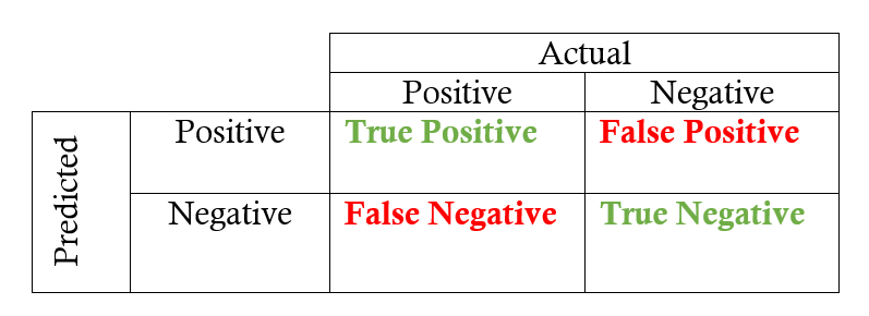
Image Source: Aditya Mishra, Medium
For a binary problem, the confusion matrix provides complete information about the model‘s performance. We can derive many metrics from these four values.
As an example, consider a model predicting whether a patient has diabetes, trained and tested on a dataset of 1000 patients, 20% of whom have diabetes. The model‘s confusion matrix on a test set is:
| Predicted Positive | Predicted Negative | |
|---|---|---|
| Actual Positive | 80 (TP) | 20 (FN) |
| Actual Negative | 40 (FP) | 860 (TN) |
We‘ll refer back to this example throughout the article.
Accuracy: A Good Starting Point, But Often Misleading
Accuracy is the fraction of examples a model classifies correctly:
$$ \text{Accuracy} = \frac{TP + TN}{TP + TN + FP + FN} $$
In our example, the model‘s accuracy is (80 + 860) / 1000 = 0.94.
While 94% accuracy may seem impressive, it can be misleading on imbalanced datasets like this one, where the positive class (diabetes) is much rarer. A naive model that always predicts "no diabetes" would achieve 90% accuracy!
This highlights the danger of using accuracy as the sole metric, especially for problems where the minority class is of greater interest or importance. Accuracy is a good starting point, but we need to dig deeper to truly assess a model‘s performance.
Precision and Recall: Focusing on Positive Predictions
Precision and recall are two metrics that provide more insight into a model‘s performance on the positive class. Precision measures the fraction of positive predictions that are correct, while recall measures the fraction of actual positives that are correctly predicted.
$$ \text{Precision} = \frac{TP}{TP + FP} $$
$$ \text{Recall} = \frac{TP}{TP + FN} $$
In our example:
- Precision = 80 / (80 + 40) = 0.667
- Recall = 80 / (80 + 20) = 0.80
The model identifies 80% of patients with diabetes (high recall), but only 66.7% of its diabetes predictions are correct (lower precision).
Precision and recall are often inversely related. Increasing the model‘s prediction threshold (the probability above which it predicts diabetes) will generally increase precision but decrease recall. This tradeoff is a key consideration in model tuning.

Image Source: Neptune.ai
The choice of whether to optimize for precision or recall (or a balance) depends on the problem. In medical diagnosis, high recall is often prioritized to avoid missing cases. In spam detection, high precision is key to avoid flagging legitimate emails. Understanding the costs and consequences of each type of error is crucial.
Thresholding and Calibration: Tuning Your Model‘s Predictions
Classification models typically output predicted probabilities, which are then thresholded to make crisp class assignments. The choice of threshold is a key lever for trading off precision and recall.

Image Source: Neptune.ai
One way to choose a threshold is to plot precision and recall as a function of the threshold and choose a value that achieves the desired balance. This requires having a well-calibrated model, where the predicted probabilities are meaningful.
Calibration plots, which bin examples by predicted probability and plot the average predicted probability against the empirical fraction of positives in each bin, are a useful diagnostic tool. A perfectly calibrated model will have all points along the diagonal line.
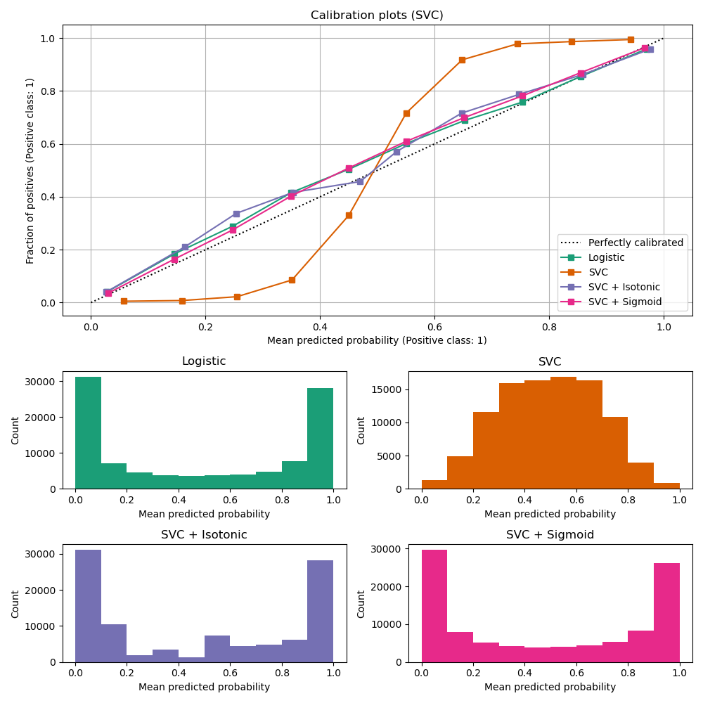
Image Source: scikit-learn
Techniques like Platt scaling and isotonic regression can help calibrate model probabilities. Well-calibrated probabilities enable more effective thresholding and provide a measure of model uncertainty.
The F1 Score: Balancing Precision and Recall
The F1 score is the harmonic mean of precision and recall, providing a single metric that balances both:
$$ F_1 = 2 \cdot \frac{\text{precision} \cdot \text{recall}}{\text{precision} + \text{recall}} $$
In our example, the F1 score is:
$$ F_1 = 2 \cdot \frac{0.667 \cdot 0.80}{0.667 + 0.80} = 0.727 $$
The F1 score is useful when you want to balance precision and recall, and there‘s no clear business reason to favor one over the other. It‘s a good default metric for binary classification problems.
AUC-ROC: A Threshold-Independent Performance Measure
The metrics we‘ve discussed so far depend on the chosen prediction threshold. An alternative approach is to evaluate the model‘s performance across all possible thresholds using the Area Under the Receiver Operating Characteristic Curve (AUC-ROC).
The ROC curve plots the True Positive Rate (recall) against the False Positive Rate (1 – specificity) at different thresholds. A perfect model hugs the top-left corner, while a random model is a diagonal line. The area under this curve (AUC) measures the model‘s ability to discriminate between classes.

Image Source: AWS
AUC ranges from 0 to 1, with 0.5 being no better than random guessing. It has an intuitive interpretation: it‘s the probability that the model ranks a random positive example higher than a random negative example.
AUC is a useful metric for comparing models, as it‘s independent of the threshold. It‘s also robust to class imbalance, since it considers all possible thresholds. However, it doesn‘t provide insight into the model‘s performance at any specific threshold.
True Negative Metrics: Specificity and Negative Predictive Value
While precision and recall focus on the model‘s performance on the positive class, specificity and negative predictive value (NPV) measure its ability to correctly identify negatives.
Specificity is the fraction of actual negatives that are correctly predicted:
$$ \text{Specificity} = \frac{TN}{TN + FP} $$
NPV is the fraction of negative predictions that are correct:
$$ \text{NPV} = \frac{TN}{TN + FN} $$
In our example:
- Specificity = 860 / (860 + 40) = 0.956
- NPV = 860 / (860 + 20) = 0.977
A model with high specificity and NPV can reliably rule out the positive class. This is important in applications like medical diagnosis, where false negatives can be costly.
Choosing the Right Metric(s) for Your Problem
With all these metrics to choose from, how do you decide which to use? The key is to consider the problem you‘re solving and the relative costs of different types of errors.
Some examples:
- In fraud detection, false positives (blocking legitimate transactions) can frustrate customers, so precision is important. But false negatives (approving fraudulent transactions) are also costly, so a balance of precision and recall (F1) may be appropriate.
- In medical diagnosis, false negatives (missing a disease) can be life-threatening, so recall is critical. Specificity is also important for avoiding unnecessary treatments.
- In ad click prediction, if ad impressions are cheap, recall may be more important than precision for showing relevant ads to users who may click.
As a general guideline:
- Start with accuracy to get a sense of overall performance, but don‘t stop there, especially for imbalanced data.
- Consider the relative costs of false positives and false negatives. Choose a metric that reflects those costs (precision, recall, specificity, NPV).
- If there‘s no clear reason to favor precision or recall, use the F1 score as a balanced metric.
- Use AUC-ROC for model comparison, especially if you‘re not sure what threshold you‘ll ultimately use.
- Always consider multiple metrics and dig into the confusion matrix to get a complete picture of your model‘s performance.
Advanced Techniques and Considerations
While the metrics we‘ve covered are a solid foundation, there are many more advanced techniques and considerations in model evaluation:
- Cost-sensitive learning: Techniques for explicitly incorporating the costs of different types of errors into model training and evaluation.
- Statistical significance: Methods for determining whether differences in metrics between models are statistically meaningful, given the size and variability of the test set.
- Confidence intervals: Techniques for quantifying the uncertainty in metric estimates, especially for small test sets.
- Cross-validation: Using multiple train/test splits to get more robust estimates of model performance.
- Multi-class metrics: Extensions of binary metrics to problems with more than two classes, such as micro- and macro-averaging.
- Regression metrics: Measures for evaluating models that predict continuous values, such as mean squared error and R-squared.
- Ranking metrics: Measures for evaluating the quality of a ranked list of results, such as precision@k and mean average precision.
Each of these topics warrants a deep dive of its own, but being aware of them will help you navigate more complex evaluation scenarios.
Current Research and Future Directions
Model evaluation is an active area of research in machine learning. Some current directions include:
- Robust and Explainable Metrics: Developing metrics that are robust to data shift and can be explained in terms of model strengths and weaknesses.
- Human-in-the-Loop Evaluation: Combining human judgment with automated metrics to get a more complete picture of model performance, especially for complex tasks.
- Domain-Specific Metrics: Developing specialized metrics for specific application domains, such as healthcare, finance, and natural language processing.
- Evaluation for Unsupervised Learning: Extending evaluation techniques to unsupervised settings like clustering and anomaly detection, where there are no ground-truth labels.
As machine learning is applied to an ever-expanding set of domains, robust and insightful evaluation will only become more important.
Conclusion: Evaluation as a Cornerstone of Effective Machine Learning
Evaluation metrics are a key tool for assessing and improving machine learning models. By understanding the strengths and weaknesses of different metrics, and how to choose the right ones for a given problem, you can more effectively develop models that meet your goals.
Remember, evaluation is not a one-time event, but an ongoing process. As you iterate on your models, continuously assess their performance using multiple metrics, dig into errors to understand their patterns, and use those insights to guide improvements.
Effective evaluation is a cornerstone of successful machine learning practice. By mastering these techniques, you‘ll be well-equipped to develop models that drive real impact.