Automate Your Excel Reports and Models with Dynamic Ranges

If you work with data in Microsoft Excel on a regular basis, you‘ve likely encountered the headache of updating charts, pivot tables, and other elements whenever your source data changes. Many analysts fall into the trap of hard-coding ranges, only to have their beautiful reports break the moment rows or columns are added or deleted in the underlying data.

Failing to plan for changes in your data sources creates a maintenance nightmare and introduces risk every time you need to refresh a report. Fortunately, by leveraging dynamic named ranges in Excel, you can build robust, low-maintenance models and automate much of your recurring reporting.

But the benefits of dynamic ranges go beyond just flexibility. They also enable you to leverage more advanced AI and machine learning capabilities in Excel to truly automate your reporting and analytics. By combining dynamic ranges with Excel‘s built-in AI functions and add-ins like Ideas, you can generate powerful insights and visualizations from your data in just a few clicks.

In this guide, we‘ll walk through multiple techniques for defining dynamic ranges, share some best practices for automating your Excel reports and models, and explore how dynamic ranges + AI can take your Excel reporting to the next level. But first, let‘s take a closer look at some of the problems caused by relying on static ranges.

The Pitfalls of Static Ranges in Excel

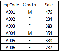
To illustrate how using fixed ranges can cause issues, consider the following simple example. Suppose you have a basic dataset showing sales by employee, like this:

EmpCode	Name	Sales
A001	John Smith	$52,000
A002	Jane Doe	$71,000
A003	Bob Johnson	$38,000

You‘ve been asked to build a quick report that includes a pivot table showing total sales by employee name, as well as a column chart visualizing the sales amounts. So you put together the following:

[Insert screenshot of basic pivot table and chart]

This looks great! The pivot and chart are linked directly to the data in cells A1:C4. You send it off, but a week later, your colleague makes some updates:

EmpCode	Name	Sales
A001	John Smith	$52,000
A002	Jane Doe	$84,000
A003	Bob Johnson	$38,000
A004	Sally Jones	$46,000

Uh oh. Now your beautiful report is broken. The new employee isn‘t included, and worse, the sales amount for Jane Doe hasn‘t updated in the pivot table or chart. The problem is you linked everything to a fixed range (A1:C4), so nothing beyond those cells is being included.

Sadly, this is an all too common issue. According to a survey by Ventana Research, 44% of enterprise spreadsheets have errors, and many can be attributed to issues with manual updating and maintenance of reports and models with hard-coded ranges and formulas.

Some analysts try to mitigate this risk by building in extra buffer rows, but this is clunky and can impact file size and performance. A study by ICAEW found that poor spreadsheet practices cost businesses an average of $55 million per year in avoidable errors and lost productivity.

The good news is there are easy ways to make your ranges dynamic in Excel so they expand and contract automatically as the size and shape of your data evolves. Let‘s explore a few of the best methods.

Create Dynamic Ranges with Excel Tables

Perhaps the simplest way to achieve dynamically updating ranges is to use Excel tables. This feature, introduced in Excel 2007, automatically applies formatting, formulas, and filters to new rows and columns added to the defined table range.

To convert your existing data range to a table:

1. Select the range, including the header row
2. Go to the Insert tab on the ribbon
3. Click the Table button
4. Verify the range and check the "My table has headers" box
5. Click OK

[Insert screenshot of creating table]

That‘s it! Your range is now an Excel table. Any charts or pivot tables you create from this table will automatically expand to include new rows or columns.

Excel tables have some other handy benefits too:

• They support structured references to make formulas more readable (e.g. =SUM(Table1[Sales])
• They automatically apply formatting and styles to new data
• They include a Total Row option for quick aggregations and calculations
• They are required for some of Excel‘s advanced AI-powered features like Ideas (more on this later)

Tables are a great option if you have a simple, contiguous data range. But in some cases, you may need more flexibility and control over your ranges. That‘s where dynamic named ranges come in.

Define Dynamic Named Ranges with INDEX, MATCH, OFFSET, and COUNTA

Creating dynamic named ranges using Excel formulas gives you the ultimate control over how your ranges resize and enables some powerful automation scenarios. The core concept is to use formulas that output a range address string that automatically adjusts based on the current size and location of your data.

Some of the key functions to master for dynamic ranges are:

• INDEX: Returns a reference to a cell at the intersection of a specific row and column
• MATCH: Locates the position of a lookup value in a row, column, or table
• OFFSET: Returns a reference shifted a specified number of rows and columns from a starting cell
• COUNTA: Counts the number of non-empty cells in a range

By combining these functions in creative ways, you can build dynamic ranges that automatically find the beginning, end, and dimensions of your data tables.

For example, here‘s a formula to create a dynamic range called "myTable" that expands or contracts to include all contiguous data starting in cell A1 on Sheet1:

=INDEX(Sheet1!$A:$Z,1,1):INDEX(Sheet1!$A:$Z,MATCH("zzz",Sheet1!$A:$A),MATCH("zzz",Sheet1!1:1,0))

This looks complex, but here‘s a breakdown:

• INDEX(Sheet1!$A:$Z,1,1): Start the range at cell A1 on Sheet1
• :: Create a range reference from the start cell to…
• INDEX(Sheet1!$A:$Z,…: On Sheet1…
• MATCH("zzz",Sheet1!$A:$A): Find the row number of the last non-empty cell in column A
• ,MATCH("zzz",Sheet1!1:1,0)): Find the column number of the last non-empty cell in row 1
• ): Close the INDEX function to return the cell at the last row and last column of data

To use this, simply go to the Name Manager on the Formulas tab, define a new name, and enter the formula in the "Refers to:" box.

[Insert screenshot of Name Manager]

Now you can use "myTable" in your pivots, charts, and formulas, and it will automatically expand or shrink when you refresh or open the workbook.

This example finds the last row and column based on any data. But you can get more targeted as well. Here‘s a formula to create a dynamic range that expands based on a specific value in column A, which is useful for things like transaction details:

=OFFSET(Sheet1!$A$1,MATCH("Total",Sheet1!$A:$A,0)-1,0,MATCH("Total",Sheet1!$A:$A,0)-1,COUNTA(Sheet1!$1:$1))

In this case, the range starts at A1 and extends to the row above the cell containing "Total" in column A, and across to the last used column in row 1.

The possibilities are endless. You can use these functions to create dynamic ranges for data tables, block references, multi-region ranges, and more. For a comprehensive list of advanced dynamic range formulas, check out this guide from ExcelJet.

Automate Your Excel Models and Reports with AI

Dynamic named ranges are a powerful tool for automating Excel reports. But when you combine them with Excel‘s built-in AI and machine learning capabilities, you can take your automation to a whole new level.

One of the easiest ways to get started with AI in Excel is with the Ideas feature. Powered by machine learning, Ideas analyzes your data and automatically generates interesting visuals, pivot tables, and insights. And it works seamlessly with Excel tables and dynamic ranges.

Here‘s a quick demo of how you can use Ideas with the dynamic range we set up earlier:

1. Make sure your data is in an Excel table (Insert tab > Table)
2. With the table selected, go to the Home tab and click the Ideas button
3. Excel will analyze your data and display some recommended charts and pivot tables
4. Hover over a card and click Insert to add the visual to your worksheet

[Insert GIF of Ideas looking at sales data and generating a chart]

Pretty slick, right? With just a few clicks, we got a nice chart showing sales by employee. And if we add data to the table, the visual will update automatically.

But Ideas is just the tip of the iceberg. Excel has a ton of other built-in AI functions that can help automate different reporting and modeling scenarios:

• FORECAST formulas use historical data to predict future values
• ANOMALY functions detect and remove outliers in data sets
• Fuzzymatch add-in uses ML to detect and fix misspellings and inconsistencies
• PowerPivot and Power Query can build complex data models and reports that refresh automatically

And the future is even brighter. Microsoft is heavily investing in AI capabilities for Excel as part of its Fluid Framework initiative. Soon you‘ll be able to use natural language queries to ask questions about your data, automatically build machine learning models, and generate entire reports from scratch, all within Excel.

In fact, in the latest release of Excel, there‘s a new LAMBDA function that lets you define your own reusable functions. When combined with dynamic ranges and other AI capabilities, you could create fully automated reporting systems, like this sales report generator:

=LAMBDA(date,
LET(data,FILTER(salesTable,(MONTH(salesTable[Date])=MONTH(date))*(YEAR(salesTable[Date])=YEAR(date))),
     salesTotal,SUM(data[Amount]),
     topRep,INDEX(data[Rep],MATCH(MAX(data[Amount]),data[Amount],0)),
     repAvg,ROUND(AVERAGE(data[Amount]),2),
RETURN("Sales Report for "&TEXT(date,"MMM YYYY")&"
Total Sales: "&TEXT(salesTotal,"$#,##0")&"
Top Rep: "&topRep&"
Average per Rep: "&TEXT(repAvg,"$#,##0")))
)

This code snippet uses the new LAMBDA function along with LET and several dynamic range formulas to build a full sales report just by passing in a date input. And this could be automatically refreshed each month using Power Automate.

The point is, AI and automation are the future of reporting in Excel. And dynamic ranges are the key to unlocking their full potential. By using the techniques and formulas we‘ve covered in this guide, you‘ll be ready to take advantage of all the powerful AI capabilities that Excel has to offer, both now and in the coming years.

Conclusion

At this point, I hope you have a solid grasp of how dynamic ranges can help you automate your Excel reports and unlock powerful AI-assisted insights. We‘ve covered a lot of ground, from the pitfalls of static ranges to advanced dynamic range formulas to practical examples of AI-powered automation with Ideas, LAMBDA, and other tools.

It‘s tempting to just brute force your way through building an Excel report. Quickly throw some data together, hit a few clicks to make a chart, and call it done. But if you invest just a bit more time to set up dynamic ranges and leverage Excel‘s built-in AI capabilities, you can build flexible models and automated reporting systems that save massive time and effort in the long run.

No more manually updating ranges and inputs each time you refresh your reports. No more playing whack-a-mole to find and fix errors caused by hard-coded formulas and bad references. No more starting from scratch each time you need to create a similar report or run a new analysis.

With dynamic ranges and AI, you can create Excel models that update themselves, PivotTable reports that generate their own insights, and complex data models that refresh and expand automatically as your data grows. All of which frees you up to focus on what matters most – making decisions and driving your business forward with confidence.

So go forth and automate! Your future self will thank you. And who knows, with all the time you save, maybe you can finally take that vacation you‘ve been putting off for "just one more report."