A Beginner‘s Guide to Time Series Modeling with Auto ARIMAX

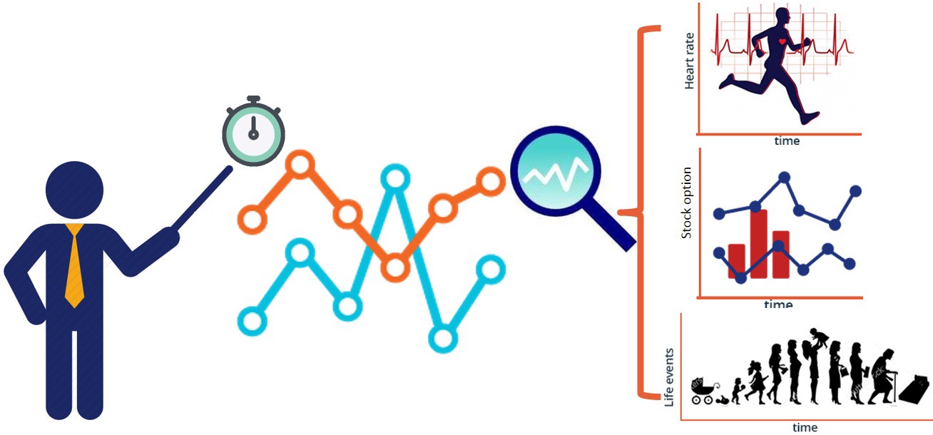
Time series data and analysis are ubiquitous in fields like business, economics, finance, and many of the sciences. A time series is a sequence of data points collected and recorded sequentially over time. Examples include daily stock prices, monthly sales figures, annual global temperatures, and countless other metrics measured at regular time intervals.

The goal of time series analysis is to extract meaningful insights from this temporal data and forecast likely future values. However, time series introduce unique challenges compared to other types of data due to the inherent time dependency between observations.

In this article, we‘ll explore one of the most widely used approaches to time series modeling – Auto Regressive Integrated Moving Average with Explanatory Variables (Auto ARIMAX). By the end, you‘ll understand the key concepts behind this technique and how to implement it yourself in Python. Let‘s dive in!

The Building Blocks of Time Series

Before we get into the details of ARIMAX models, it‘s important to understand the main components that constitute a time series:

1. Trend: The overall upward or downward movement of the data over time. Trends can be linear or non-linear.

2. Seasonality: Recurring patterns or cycles of highs and lows related to calendar-based factors like the time of year or day of the week.

3. Cyclical: Rises and falls not of fixed period. These fluctuations are usually due to economic conditions and are often unpredictable.

4. Irregular: The residual, random noise left over after accounting for the other 3 components. Irregularity is unpredictable.

Most time series will contain a mix of some or all of these elements. The first step in many time series modeling tasks is to deconstruct the series into these constituent parts.

Stationarity – A Key Assumption

Another critical concept in time series analysis is stationarity. A stationary time series is one whose statistical properties like the mean and variance are constant over time. Most time series models, including those in the ARIMA family, assume stationarity.

Unfortunately, most real-world time series are non-stationary. They often contain trends and seasonal patterns that violate the constant mean and variance assumptions. The good news is we can often transform a non-stationary series to be stationary through differencing.

Differencing means computing the differences between consecutive observations. The first difference is simply the series of changes from one time period to the next. We can difference the data as many times as needed to achieve stationarity. The number of differencing steps is captured in the "integrated" (I) term of an ARIMA model.

Autoregressive (AR) Models

With those foundations in place, let‘s now turn our attention to the first pillar of ARIMA models – autoregression (AR). An autoregressive model predicts future values based on a linear combination of past values.

The term "auto" indicates that it is a regression of the variable against itself. An AR model of order p refers to a model that uses the p most recent time periods as predictors. This can be expressed mathematically as:

y_t = c + φ₁y_t-1 + φ₂y_t-2 + … + φ_py_t-p + ε_t

where y_t is the value at time t, φ(1)…φ(p) are the parameters of the model, c is a constant, and ε_t is white noise.

Moving Average (MA) Models

The second component of an ARIMA model is the moving average (MA) model. While an AR model uses past values to predict the future, an MA model uses past forecast errors.

An MA model of order q uses the q most recent forecast errors in the following form:

y_t = c + θ₁ε_t-1 + θ₂ε_t-2 + … + θ_qε_t-q + ε_t

Here θ(1)…θ(q) are the parameters of the model, and ε_t-i is the forecast error at time t-i.

ARIMA – Putting it All Together

As the name suggests, an ARIMA model combines these AR and MA components along with differencing. The full model can be written as:

y^‘_t = c + φ₁y^‘_t-1 + … + φ_py^‘_t-p + θ₁ε_t-1 + … + θ_qε_t-q + ε_t

where y^‘_t is the differenced series.

The values of p, d, and q are the three main hyperparameters of the model that together specify the order. For example, an ARIMA(1,1,0) model contains one AR term, one differencing step, and zero MA terms.

Introducing Exogenous Variables with ARIMAX

A pure ARIMA model assumes that the future values of a series depend only on its own past values and past forecast errors. However, in many real-world scenarios, we have additional independent variables that can help explain the behavior of our time series. These are called exogenous variables.

An ARIMAX model extends ARIMA to incorporate exogenous variables. This allows the model to capture how changes in external factors like pricing, marketing spend, economic indicators, etc. are likely to impact the forecast.

Exogenous variables can be continuous or categorical, and are incorporated into the ARIMA equation as additional regression terms. The model learns coefficients for each exogenous variable that describe the size and direction of its effect.

Automating Model Selection with Auto ARIMAX

We‘ve now covered the theoretical components that make up an ARIMAX model. But how do we choose optimal values for the p, d, and q order terms and which exogenous variables to include?

Traditionally, this required manually fitting and comparing many different models which could be very time consuming. Fortunately, more recent implementations like the auto_arima function from the pmdarima Python package allow us to automate much of this process.

Auto ARIMAX will automatically perform the differencing required to make the series stationary and then conduct a search across different combinations of p and q values. It selects the best model based on an information criterion like AIC which balances goodness of fit against model complexity.

We simply provide the training data and a list of exogenous variables we want to consider. The algorithm handles the rest!

A Practical Example

Let‘s make these concepts concrete with a worked example in Python. We‘ll use a dataset of historical daily stock prices for a major financial services company and attempt to forecast future prices using an auto ARIMAX model.

We start by importing our data and creating a dataframe with the date as the index:

df = pd.read_csv("stock_data.csv") 
df.set_index("Date", drop=False, inplace=True)

Next we generate some features to use as exogenous variables. In this case, we calculate rolling averages and standard deviations of key stock indicators like price and trading volume over different lookback periods to capture recent trends. We also include categorical variables for calendar-based seasonality.

lag_features = ["High", "Low", "Volume", "Turnover", "Trades"]
window1 = 3
window2 = 7 
window3 = 30

df_rolled_3d = df[lag_features].rolling(window=window1, min_periods=0)
df_mean_3d = df_rolled_3d.mean().shift(1).reset_index().astype(np.float32)
df_std_3d = df_rolled_3d.std().shift(1).reset_index().astype(np.float32)

# Repeat for 7 and 30 day windows

for feature in lag_features:
    df[f"{feature}_mean_lag{window1}"] = df_mean_3d[feature]
    df[f"{feature}_std_lag{window1}"] = df_std_3d[feature]

    # Repeat for 7 and 30 day windows

df.Date = pd.to_datetime(df.Date, format="%Y-%m-%d")
df["month"] = df.Date.dt.month
df["week"] = df.Date.dt.week
df["day"] = df.Date.dt.day
df["day_of_week"] = df.Date.dt.dayofweek

We then split our data into train and test sets. The model will be trained on data from 2008-2018 and we‘ll generate forecasts for 2019.

df_train = df[df.Date < "2019"]
df_valid = df[df.Date >= "2019"]

Now we‘re ready to train our Auto ARIMAX model. We provide the training data, specify the exogenous features, and the model does the rest.

exogenous_features = [...]

model = auto_arima(df_train.VWAP, exogenous=df_train[exogenous_features], 
                   trace=True, error_action="ignore", suppress_warnings=True)

model.fit(df_train.VWAP, exogenous=df_train[exogenous_features])

Once trained, we can generate forecasts for our validation period. The number of periods to forecast is set by n_periods and we provide the exogenous variable values for this future period.

forecast = model.predict(n_periods=len(df_valid), exogenous=df_valid[exogenous_features])

Finally, we evaluate the performance of our model by comparing the forecasted values to the actual values. Two common metrics for this are Root Mean Squared Error (RMSE) and Mean Absolute Error (MAE).

print("RMSE of Auto ARIMAX:", np.sqrt(mean_squared_error(df_valid.VWAP, forecast)))
print("MAE of Auto ARIMAX:", mean_absolute_error(df_valid.VWAP, forecast))

In this case, our Auto ARIMAX model achieves an RMSE of around 147 and MAE of 104 on the validation set which seems reasonable. We can also plot the forecast against the actual values to visually assess the fit.

Limitations and Alternatives

While Auto ARIMAX is a powerful and widely used technique, it‘s important to be aware of its limitations. ARIMAX models assume linear relationships which may not always hold in reality. They can also struggle with very long-term dependencies and abrupt changes in the level of the series.

For highly non-linear or complex series, methods like recurrent neural networks (RNNs) and in particular LSTMs may be more suitable. Another alternative is Facebook‘s Prophet library which is designed for business time series with strong seasonality.

Ultimately, the best approach will depend on the characteristics of your data and the specific requirements of your use case. It‘s often valuable to experiment with multiple methods and compare their empirical performance.

Conclusion

We‘ve covered a lot of ground in this guide to time series modeling with Auto ARIMAX. We started with the fundamentals of what makes time series unique and how to decompose them into trend, seasonal, and irregular components.

We then introduced the idea of stationarity and saw how differencing can be used to make a series stationary. Next, we examined the autoregressive and moving average components that form the building blocks of ARIMA models.

Building on this, we saw how ARIMAX extends ARIMA to incorporate exogenous variables and how the auto_arima function enables us to automate the process of finding the optimal model order and parameters.

We then walked through a complete example of training an Auto ARIMAX model to forecast stock prices and evaluated its performance. Finally, we discussed some limitations of ARIMAX and alternative approaches.

Time series modeling is a vast field and we‘ve only scratched the surface here. But armed with an understanding of these key concepts, you‘re well positioned to start applying Auto ARIMAX to your own time series problems. I encourage you to experiment with the code examples and test your new knowledge on other datasets.

As you do so, always remember that while powerful, no model is perfect. The real world is messy and complex, and even the best models are simplifications. Always sense check your results and know that multiple models can often be used in tandem.

Happy forecasting!