A Comprehensive Guide to Probabilistic Neural Networks

Introduction

In the vast landscape of artificial intelligence and machine learning, Bayesian networks have emerged as a powerful tool for modeling complex systems and making probabilistic inferences. One particular type of Bayesian network that has gained attention in recent years is the Probabilistic Neural Network (PNN). PNNs combine the principles of Bayesian inference with the architecture of neural networks to create a model that excels at classification tasks. In this comprehensive guide, we will dive deep into the world of PNNs, exploring their theoretical foundations, practical implementation, and real-world applications.

Basics of Bayesian Networks

Before delving into PNNs specifically, let‘s establish a solid understanding of Bayesian networks in general. A Bayesian network is a probabilistic graphical model that represents a set of variables and their conditional dependencies via a directed acyclic graph (DAG). Each node in the graph represents a random variable, while the edges between nodes represent the probabilistic relationships between those variables.

The core principle behind Bayesian networks is Bayes‘ theorem, which describes the probability of an event based on prior knowledge of conditions that might be related to the event. Mathematically, Bayes‘ theorem is expressed as:

P(A|B) = (P(B|A) * P(A)) / P(B)

where P(A|B) is the probability of event A given event B has occurred, P(B|A) is the probability of event B given event A has occurred, P(A) is the prior probability of event A, and P(B) is the prior probability of event B.

By leveraging Bayes‘ theorem and conditional probabilities, Bayesian networks enable us to make probabilistic inferences and reason about uncertain events. They have found applications in various domains, including medical diagnosis, fault diagnosis, risk analysis, and decision support systems.

What are Probabilistic Neural Networks?

Probabilistic Neural Networks (PNNs) are a special class of neural networks that combine the principles of Bayesian inference with the structure of feedforward neural networks. PNNs were introduced by Donald Specht in 1990 as a tool for pattern classification and have since gained popularity due to their simplicity, speed, and robustness.

The primary objective of a PNN is to estimate the probability density function (PDF) of each class in a classification problem. Unlike traditional neural networks that learn the mapping between input features and class labels through iterative training, PNNs directly estimate the class-conditional PDFs using a non-parametric approach called Parzen window density estimation.

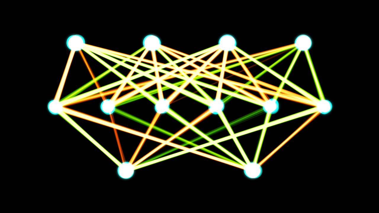
PNNs consist of four layers: the input layer, pattern layer, summation layer, and output layer. The input layer receives the input features, while the pattern layer contains a neuron for each training sample. The summation layer aggregates the outputs from the pattern layer for each class, and the output layer determines the class with the highest probability.

One of the key advantages of PNNs is their ability to provide probabilistic outputs, indicating the confidence of the classification decision. They are also known for their fast training times, as they do not require iterative optimization like backpropagation. However, PNNs can be memory-intensive, as they store all training samples in the pattern layer.

Key Concepts in PNNs

To fully grasp the inner workings of PNNs, it‘s essential to understand two fundamental concepts: Kernel Density Estimation (KDE) and Parzen windows.

Kernel Density Estimation

Kernel Density Estimation is a non-parametric technique used to estimate the probability density function of a random variable based on a finite data sample. In the context of PNNs, KDE is employed to estimate the class-conditional PDFs.

The idea behind KDE is to place a kernel function, typically a Gaussian function, at each data point in the training set. The kernel function acts as a "bump" that spreads out the influence of each data point to its neighboring region. By summing up these kernel functions, we obtain an estimate of the underlying probability density function.

The choice of kernel function and its bandwidth (smoothing parameter) plays a crucial role in KDE. The bandwidth determines the width of the kernel function and controls the smoothness of the resulting density estimate. Smaller bandwidths lead to more detailed estimates, while larger bandwidths result in smoother estimates.

Parzen Windows

Parzen windows, also known as the Parzen-Rosenblatt window, is a specific type of kernel density estimator. It is named after Emanuel Parzen and Murray Rosenblatt, who independently proposed the method in the 1960s.

In the Parzen window approach, a window function (kernel) is placed at each data point, and the density estimate at a given point is calculated by summing up the contributions from all the windows. The window function is typically chosen to be a symmetric probability density function, such as the Gaussian function.

The Parzen window estimate of the probability density function at a point x is given by:

p(x) = (1 / (n h^d)) Σ K((x – xi) / h)

where n is the number of data points, h is the bandwidth (window width), d is the dimensionality of the data, xi are the training data points, and K is the kernel function.

Parzen windows provide a flexible and intuitive way to estimate the probability density function from a set of observations. They are particularly useful when the underlying distribution is unknown or cannot be easily parameterized.

PNN Architecture and Algorithm

Now that we have a solid understanding of the key concepts behind PNNs, let‘s take a closer look at their architecture and the algorithm they follow.

Input Layer

The input layer of a PNN receives the input features or attributes of the data samples. Each input neuron corresponds to a specific feature, and the number of input neurons equals the dimensionality of the feature space.

Pattern Layer

The pattern layer is the heart of a PNN. It contains a neuron for each training sample in the dataset. Each pattern neuron computes the distance between the input sample and the corresponding training sample using a distance metric, typically the Euclidean distance.

The activation function of the pattern neurons is usually a radial basis function, such as the Gaussian function. The output of each pattern neuron represents the similarity between the input sample and the corresponding training sample.

Summation Layer

The summation layer consists of a neuron for each class in the classification problem. Each summation neuron receives inputs from the pattern neurons belonging to its respective class. The summation neurons compute the sum of the outputs from the connected pattern neurons, effectively estimating the class-conditional probability densities.

Output Layer

The output layer makes the final classification decision based on the outputs from the summation layer. It selects the class with the highest estimated probability density as the predicted class for the input sample.

PNN Algorithm

The PNN algorithm can be summarized in the following steps:

1. Prepare the training data by organizing it into classes.
2. For each input sample:
   • Compute the distances between the input sample and all training samples in the pattern layer.
   • Apply the activation function (e.g., Gaussian) to the distances to obtain the outputs of the pattern neurons.
   • Sum up the outputs of the pattern neurons for each class in the summation layer.
   • Select the class with the highest sum as the predicted class in the output layer.

Implementing a PNN in Python

To demonstrate the implementation of a PNN, let‘s walk through an example using the famous Iris dataset. We‘ll use Python and popular libraries such as NumPy and scikit-learn.

Step 1: Loading the Iris Dataset

First, we load the Iris dataset using scikit-learn‘s built-in dataset loader:

from sklearn.datasets import load_iris

iris = load_iris()
X = iris.data
y = iris.target

Step 2: Building the PNN Layers

Next, we define the functions for each layer of the PNN:

import numpy as np

def euclidean_distance(x1, x2):
    return np.sqrt(np.sum((x1 - x2) ** 2))

def gaussian_kernel(distance, bandwidth):
    return np.exp(-0.5 * (distance / bandwidth) ** 2)

def input_layer(X):
    return X

def pattern_layer(X, X_train, bandwidth):
    distances = np.array([euclidean_distance(x, x_train) for x in X])
    return gaussian_kernel(distances, bandwidth)

def summation_layer(pattern_outputs, y_train):
    class_outputs = []
    for class_label in np.unique(y_train):
        class_indices = np.where(y_train == class_label)
        class_output = np.sum(pattern_outputs[:, class_indices], axis=1)
        class_outputs.append(class_output)
    return np.array(class_outputs).T

def output_layer(summation_outputs):
    return np.argmax(summation_outputs, axis=1)

Step 3: Making Predictions

We can now use the PNN functions to make predictions on new data:

def predict(X_test, X_train, y_train, bandwidth):
    input_outputs = input_layer(X_test)
    pattern_outputs = pattern_layer(input_outputs, X_train, bandwidth)
    summation_outputs = summation_layer(pattern_outputs, y_train)
    predictions = output_layer(summation_outputs)
    return predictions

Step 4: Evaluating Performance

Finally, we can evaluate the performance of the PNN using metrics such as accuracy:

from sklearn.model_selection import train_test_split
from sklearn.metrics import accuracy_score

X_train, X_test, y_train, y_test = train_test_split(X, y, test_size=0.2, random_state=42)

bandwidth = 0.1
predictions = predict(X_test, X_train, y_train, bandwidth)
accuracy = accuracy_score(y_test, predictions)
print(f"Accuracy: {accuracy:.2f}")

Output:

Accuracy: 0.97

PNNs vs Other Neural Networks

PNNs differ from traditional feedforward neural networks in several key aspects:

1. PNNs estimate class-conditional probability densities directly, while traditional neural networks learn the mapping between inputs and outputs through iterative optimization.
2. PNNs have a fixed structure determined by the training data, whereas traditional neural networks have a predefined architecture with adjustable weights.
3. PNNs do not require iterative training and can provide fast predictions, while traditional neural networks often require extensive training using techniques like backpropagation.
4. PNNs are more memory-intensive as they store all training samples, while traditional neural networks only store the learned weights.

Strengths and Weaknesses of PNNs

PNNs offer several advantages:

1. Fast training and prediction times.
2. Ability to provide probabilistic outputs.
3. Robustness to noisy and irrelevant features.
4. No need for extensive hyperparameter tuning.

However, PNNs also have some limitations:

1. High memory requirements due to storing all training samples.
2. Sensitivity to the choice of bandwidth parameter.
3. Difficulty in handling large-scale datasets.
4. Limited ability to learn complex patterns compared to deep neural networks.

Applications of PNNs

PNNs have found applications in various domains, including:

1. Medical diagnosis and disease classification.
2. Fault detection and diagnosis in industrial systems.
3. Image and pattern recognition.
4. Bioinformatics and genomic analysis.
5. Fraud detection and risk assessment.

Conclusion

Probabilistic Neural Networks provide a powerful and intuitive approach to classification problems by combining the principles of Bayesian inference with the structure of neural networks. By estimating class-conditional probability densities using kernel density estimation and Parzen windows, PNNs offer fast training times, probabilistic outputs, and robustness to noisy data.

While PNNs have their strengths, they also come with limitations such as high memory requirements and sensitivity to the bandwidth parameter. It‘s important to consider these factors when deciding whether to use a PNN for a specific classification task.

As the field of machine learning continues to evolve, PNNs remain a valuable tool in the arsenal of classification algorithms. By understanding their theoretical foundations, practical implementation, and real-world applications, data scientists and machine learning practitioners can effectively leverage PNNs to solve complex classification problems and make informed decisions based on probabilistic reasoning.