A Deep Dive into Regression Analysis Assumptions: Plots, Solutions, and More

Regression analysis is a powerful statistical method used to model the relationship between a dependent variable and one or more independent variables. It forms the foundation of predictive modeling and is widely used across industries, from finance to healthcare to marketing.

However, running a regression model is not as simple as fitting a line to data points. There are important assumptions that must be met to ensure the model is valid and the results can be trusted. Violating these assumptions can lead to biased coefficients, unreliable p-values, and inaccurate predictions.

In this comprehensive guide, we‘ll take a deep dive into regression analysis assumptions. You‘ll learn:

• The 6 critical assumptions that must be met
• How to detect violations of each assumption using plots and tests
• Solutions and fixes for each violation
• Examples, FAQs, and more

By the end of this post, you‘ll be equipped with a solid understanding of regression assumptions and practical tools to validate your own models. Let‘s get started!

The 6 Critical Assumptions of Linear Regression

Linear regression relies on 6 key assumptions being met. If any of these assumptions are violated, the results of the model may not be valid or reliable. The assumptions are:

1. Linearity

The first and most important assumption is that the relationship between the dependent and independent variables is linear. In simple terms, this means the effect of a change in X on Y is constant, regardless of the value of X.

There are a few ways to check for linearity:

• Create a scatter plot of the dependent vs independent variables. The relationship should follow a straight line.
• Plot the residuals (actual – predicted values) vs the fitted (predicted) values. The points should be symmetrically distributed around a horizontal line.
• Include polynomial terms (x^2, x^3, etc.) in the model. If these are significant, the relationship is likely non-linear.

If the linearity assumption is violated, the model will be biased and can give misleading results. Some solutions are to:

• Transform the dependent or independent variables (log, square root, etc.)
• Use a non-linear model like polynomial regression
• Add interaction terms

2. Independence

The second assumption is that the observations (data points) are independent of each other. In other words, the value of one observation does not depend on or influence the value of another.

This is mainly an issue in time series data, where observations are naturally ordered. For example, today‘s stock price is not independent from yesterday‘s price.

Some signs that independence is violated:

• Autocorrelation (correlation between an observation and its past values)
• Seasonality or trends over time
• Clustered or hierarchical data

The most common way to test for independence is with the Durbin-Watson statistic. A value of 2 indicates no autocorrelation, while values below 2 indicate positive autocorrelation and above 2 indicate negative autocorrelation.

If independence is violated, the standard errors will be underestimated, leading to narrower confidence intervals and smaller p-values. Some solutions are to:

• Use time series models like ARIMA or VAR
• Include lagged variables as predictors
• Use clustered standard errors
• Average data over time periods

3. Homoscedasticity

Homoscedasticity means the variance of the residuals is constant across all values of the independent variables. In other words, the spread of the residuals should be roughly equal at all fitted values.

The opposite of homoscedasticity is heteroscedasticity – when the variance is unequal across the range of values. Some causes are:

• Outliers or extreme values
• Omitted variables
• Model misspecification

The easiest way to check for homoscedasticity is to plot the residuals vs fitted values. The points should be randomly and evenly dispersed with no patterns. Some formal tests are the Breusch-Pagan test and White‘s test.

If the homoscedasticity assumption is violated, the regression coefficients are still unbiased, but the standard errors and p-values may be invalid. Some solutions are to:

• Transform the dependent variable (log, square root, etc.)
• Use weighted least squares regression
• Use heteroscedasticity-robust standard errors

4. Normality of Residuals

The fourth assumption is that the residuals are normally distributed with a mean of zero. This doesn‘t mean the dependent or independent variables have to be normal – just the residuals.

Some ways to check normality:

• Create a histogram or density plot of the residuals. It should follow a bell curve.
• Use a Q-Q plot to compare the residuals to a normal distribution. The points should follow a straight diagonal line.
• Formal tests like the Shapiro-Wilk or Kolmogorov-Smirnov test

If normality is violated, the p-values and confidence intervals may be unreliable, especially for small sample sizes. Some solutions are:

• Transform the dependent or independent variables
• Use a different type of regression like quantile regression
• Use bootstrapping to estimate standard errors and confidence intervals

5. No Multicollinearity

Multicollinearity occurs when two or more independent variables are highly correlated with each other. This makes it difficult to determine which variable is actually influencing the dependent variable.

Some signs of multicollinearity:

• Very high R^2 but few significant coefficients
• Coefficients have a sign opposite of what‘s expected
• Adding or removing a variable significantly changes the coefficients

The most common ways to detect multicollinearity are:

• Create a correlation matrix of the independent variables. Correlations above 0.7-0.8 indicate a problem.
• Calculate the variance inflation factor (VIF). Values above 5-10 suggest multicollinearity.

Multicollinearity doesn‘t bias the coefficients, but it does increase the standard errors, making it hard to assess the individual impact of each predictor. Some solutions are:

• Remove one of the correlated variables
• Combine the correlated variables into a single predictor
• Use dimensionality reduction methods like PCA
• Use regularization techniques like ridge or lasso regression

6. No Endogeneity

Endogeneity means there is a correlation between the independent variable(s) and the error term. This violates the assumption that all relevant variables are included in the model and there is no systematic bias.

Some common causes of endogeneity are:

• Omitted variable bias – an important confounder is left out
• Measurement error in the independent variables
• Simultaneous causality – X causes Y but Y also causes X

Endogeneity is tricky to detect and often relies on domain knowledge rather than plots or statistics alone. Some general signs are:

• The coefficients are much larger or smaller than expected
• The model doesn‘t generalize well to out-of-sample data
• Significant changes to the coefficients when adding or removing variables

If endogeneity is present, the regression coefficients will be biased and inconsistent. Some solutions are:

• Add omitted confounders to the model, if available
• Use instrumental variables estimation
• Use fixed effects or difference-in-differences models for panel data
• Collect better quality data

How to Check Regression Assumptions

Now that we‘ve covered the 6 main assumptions, let‘s dive into how to actually validate them using plots and tests in Python. We‘ll use the built-in Boston Housing dataset as an example.

Linearity and Homoscedasticity: Residuals vs Fitted Plot

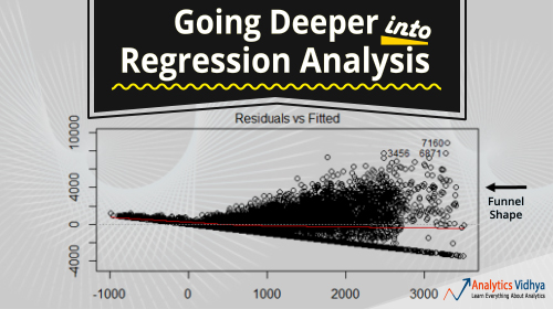
The first plot to check is a scatter plot of residuals (y-axis) vs fitted values (x-axis). This plot can diagnose violations of both linearity and homoscedasticity.

If the relationship is linear and homoscedastic, the points should be randomly scattered around the horizontal line at zero with no obvious patterns. A non-linear pattern (like a U-shape) indicates the linearity assumption is violated, while a funnel or fan shape indicates heteroscedasticity.

Here‘s how to create this plot in Python:

import statsmodels.api as sm

model = sm.OLS(y, sm.add_constant(X)).fit()

residuals = model.resid
fitted = model.fittedvalues

plt.scatter(fitted, residuals)
plt.xlabel(‘Fitted Values‘)
plt.ylabel(‘Residuals‘)
plt.axhline(y=0, color=‘r‘, linestyle=‘:‘)
plt.show()

Normality of Residuals: Q-Q Plot and Histogram

To check if the residuals are normally distributed, we can use a Q-Q plot and histogram. In the Q-Q plot, the quantiles of the residuals are plotted against the quantiles of a normal distribution. If the residuals are normal, the points will follow the diagonal line.

Here‘s the code for a Q-Q plot:

from scipy.stats import probplot

probplot(model.resid, dist=‘norm‘, plot=plt)
plt.show()

We can also plot a histogram of the residuals and visually check for a bell-shaped curve:

plt.hist(model.resid, bins=20)
plt.xlabel(‘Residuals‘)
plt.ylabel(‘Frequency‘)
plt.show() 

Independence: Durbin-Watson Test

To formally test for autocorrelation in the residuals, we can use the Durbin-Watson test. A value close to 2 indicates no autocorrelation, while a value below 1 or above 3 suggests a problem.

from statsmodels.stats.stattools import durbin_watson

print(durbin_watson(model.resid))

Multicollinearity: VIF and Correlation Matrix

To check for multicollinearity, we can calculate the variance inflation factor (VIF) for each independent variable. A VIF above 5-10 indicates a problem.

Here‘s how to do it in Python:

from statsmodels.stats.outliers_influence import variance_inflation_factor

vif = [variance_inflation_factor(X.values, i) for i in range(X.shape[1])]
print(pd.DataFrame({‘feature‘: X.columns, ‘vif‘: vif}))

We can also create a correlation matrix of the independent variables and look for any correlations above 0.7-0.8.

corr_matrix = X.corr()
print(corr_matrix)

Solutions for Violating Regression Assumptions

If any of the assumptions are violated, don‘t despair! There are solutions and fixes you can try to improve your model:

• Transform the dependent or independent variables with functions like log, square root, or reciprocal
• Use a non-linear model like polynomial regression or generalized additive models (GAM)
• Add interaction terms to capture non-linear relationships
• Use weighted least squares (WLS) regression for heteroscedasticity
• Use robust standard errors for heteroscedasticity and normality violations
• Remove outliers and influential points
• Combine or remove correlated independent variables
• Use regularization techniques like ridge or lasso regression for multicollinearity
• Add omitted variables to the model to reduce endogeneity bias
• Use instrumental variables (IV) estimation for endogeneity

Conclusion

We covered a lot of ground in this post! To recap, the 6 main assumptions of linear regression are:

1. Linearity
2. Independence
3. Homoscedasticity
4. Normality of residuals
5. No multicollinearity
6. No endogeneity

We showed how to check each assumption using plots and statistical tests, and provided solutions for when they are violated. By validating these assumptions, you can be more confident in the results and predictions of your regression models.

However, keep in mind that all models are wrong, but some are useful. Meeting the assumptions doesn‘t guarantee a perfect model, and violating them doesn‘t necessarily mean the results are useless. The key is to be aware of the assumptions, check them diligently, and interpret the results with caution.

I hope this guide gave you a deeper understanding of regression analysis assumptions and practical tools to apply to your own work. Happy modeling!

FAQs

Q: What are the consequences of violating regression assumptions?
A: Violating assumptions can lead to biased and inconsistent regression coefficients, unreliable p-values and confidence intervals, and inaccurate predictions. The severity depends on the type and degree of violation.

Q: Do I need to meet all the assumptions for my regression model to be valid?
A: While it‘s ideal to meet all the assumptions, in reality, most data will violate at least one. The goal is to minimize the severity of the violations and use appropriate fixes and robust methods. A model can still be useful even if some assumptions are not met.

Q: What if I can‘t transform my data to meet the linearity assumption?
A: If transformations don‘t work, you can try using a non-linear model like polynomial regression, GAMs, or decision trees. These models don‘t assume a linear relationship between the dependent and independent variables.

Q: How do I know which variables to include in my model to avoid omitted variable bias?
A: This is a challenge and often relies on domain knowledge and expertise. Some general tips are to consider any variables that are correlated with both the dependent and independent variables, consult with subject matter experts, and use model selection techniques like stepwise regression or regularization.

Q: Can I use regression if my data is not normally distributed?
A: The normality assumption applies to the residuals, not the raw data. However, if the dependent variable is heavily skewed or has outliers, it can affect the residuals. In this case, you can try transforming the dependent variable or using a generalized linear model (GLM) that doesn‘t assume normality.