Measuring the Spread of Data: An In-Depth Guide to Range, IQR, Variance, and Standard Deviation

Introduction

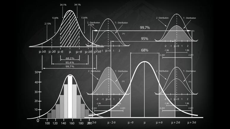
As an AI and machine learning expert, I know that understanding the dispersion or variability of a dataset is crucial for data analysis, modeling, and decision-making. Measures of dispersion quantify how much the data values are spread out from the center or from each other. They provide essential information about the distribution, consistency, and potential outliers in the data.

In this comprehensive guide, we‘ll dive deep into four fundamental measures of dispersion: range, interquartile range (IQR), variance, and standard deviation. We‘ll explore their definitions, calculations, interpretations, advantages, and disadvantages. Special attention will be given to comparing IQR and standard deviation, two of the most widely used measures.

Whether you‘re a data scientist, researcher, student, or professional working with data, this guide will equip you with a solid understanding of these important statistical tools. Let‘s get started!

Range: The Simplest Measure of Dispersion

Range is the simplest and most intuitive measure of dispersion. It is defined as the difference between the largest and smallest values in a dataset.

Mathematically, for a dataset X = {x₁, x₂, …, xₙ}:

Range = max(X) – min(X)

For example, consider the following dataset of exam scores:
X = {72, 85, 90, 68, 77, 92, 88, 83}

The range is:
max(X) – min(X) = 92 – 68 = 24

Interpretation:

• A small range indicates the data is clustered closely together.
• A large range indicates the data is more spread out.

Advantages:

• Easy to calculate and understand
• Provides a quick measure of the total spread

Disadvantages:

• Sensitive to outliers, since it only considers the two extreme values
• Doesn‘t provide any information about the dispersion of the middle portion of the data

Range is most useful as a preliminary measure of dispersion or when the full data is not available. However, it‘s important to complement it with other measures for a more complete understanding.

Interquartile Range (IQR): A Robust Measure of Dispersion

The interquartile range (IQR) is a more robust measure of dispersion that is less affected by outliers. It measures the range of the middle 50% of the data, defined as the difference between the third quartile (Q3) and the first quartile (Q1).

To calculate the IQR:

1. Arrange the data in ascending order.
2. Find the median (Q2) that divides the data into two halves.
3. Find the median of the lower half (Q1) and the upper half (Q3).
4. Calculate IQR = Q3 – Q1

For the exam scores dataset:
Sorted X = {68, 72, 77, 83, 85, 88, 90, 92}
Q1 = 74.5 (median of 68, 72, 77)
Q3 = 89 (median of 85, 88, 90, 92)
IQR = Q3 – Q1 = 89 – 74.5 = 14.5

Interpretation:

• A small IQR indicates the middle 50% of data is clustered closely.
• A large IQR indicates the middle 50% of data is more spread out.

Advantages:

• Robust to outliers, as it only considers the middle 50% of data
• Provides information about the dispersion of the central portion of the data
• Can be used to identify potential outliers (e.g. values below Q1 – 1.5×IQR or above Q3 + 1.5×IQR)

Disadvantages:

• Ignores the dispersion of the lowest 25% and highest 25% of data
• Less sensitive to changes in the tails of the distribution

IQR is particularly useful for skewed distributions or data with outliers. It‘s often used in box plots to visualize the dispersion and identify outliers.

Variance and Standard Deviation: Measuring Average Dispersion

Variance and standard deviation are the most commonly used measures of dispersion. They quantify the average squared deviation of each data point from the mean.

For a population of size N with mean μ, the population variance is:

σ² = Σ(xᵢ – μ)² / N

For a sample of size n with mean x̄, the sample variance is:

s² = Σ(xᵢ – x̄)² / (n – 1)

The standard deviation is the square root of the variance:

Population standard deviation: σ = √(σ²)
Sample standard deviation: s = √(s²)

Let‘s calculate the sample variance and standard deviation for the exam scores dataset:
n = 8, x̄ = 81.875

xᵢ	(xᵢ – x̄)²
72	97.5156
85	9.7656
90	66.0156
68	192.0156
77	23.7656
92	102.5156
88	37.5156
83	1.2656
Sum	530.3848

s² = 530.3848 / (8 – 1) = 75.7692
s = √(75.7692) = 8.7057

Interpretation:

• A small variance or standard deviation indicates the data points are clustered closely around the mean.
• A large variance or standard deviation indicates the data points are spread far from the mean.

Advantages:

• Incorporates all data points in the calculation
• Provides a precise measure of average dispersion
• Has well-defined mathematical properties and relationships to the normal distribution (empirical rule, Chebyshev‘s inequality)
• Widely used in statistical inference, hypothesis testing, and modeling

Disadvantages:

• More complex to calculate and interpret than range or IQR
• Sensitive to outliers due to squared deviations
• Assumes the data is approximately normally distributed for some interpretations

Variance and standard deviation are suitable for roughly symmetric, unimodal distributions without extreme outliers. They form the basis for many statistical techniques, such as z-scores, the Coefficient of Variation, ANOVA, and regression.

It‘s important to note the distinction between population and sample formulas. The sample variance has n-1 in the denominator (Bessel‘s correction) to account for using the sample mean instead of the usually unknown population mean. This correction makes the sample variance an unbiased estimator of the population variance.

Comparing IQR and Standard Deviation

While both IQR and standard deviation measure dispersion, they have some key differences:

Property	IQR	Standard Deviation
Definition	Q3 – Q1	√(Σ(xᵢ – x̄)² / (n – 1))
Sensitivity to outliers	Robust	Sensitive
Portion of data considered	Middle 50%	All data points
Ease of calculation	Moderate	More complex
Ease of interpretation	Easier	More complex
Relationship to distribution	Works well for skewed data	Assumes normal distribution
Mathematical properties	Limited	Well-defined
Use in statistical inference	Limited	Extensive

In general, IQR is preferred when the data is skewed, contains outliers, or when a simple, robust measure is needed. Standard deviation is preferred when the data is approximately normal, when all data points need to be considered, or when further statistical analysis is required.

However, it‘s often beneficial to calculate and compare both measures to get a more comprehensive understanding of the dispersion. Substantial differences between IQR and standard deviation can indicate skewness, heavy tails, or outliers in the data.

Visualizing Dispersion

Measures of dispersion are most informative when combined with visual representations of the data. Two common plots for visualizing dispersion are histograms and box plots.

A histogram shows the distribution of the data by dividing the range into bins and plotting the frequency or density of data points in each bin. The width of the histogram indicates the total dispersion, while the shape reveals characteristics like skewness and outliers.

A box plot (or box-and-whisker plot) summarizes the five-number summary of a dataset: minimum, Q1, median, Q3, and maximum. The box spans the IQR, with the median marked inside. The whiskers extend to the minimum and maximum (or to 1.5×IQR from the box edges, with outliers plotted separately). Box plots are especially useful for comparing the dispersion of multiple datasets.

Here‘s how to create a histogram and box plot in Python using matplotlib:

import numpy as np
import matplotlib.pyplot as plt

scores = [72, 85, 90, 68, 77, 92, 88, 83]

plt.figure(figsize=(10, 4))

# Histogram
plt.subplot(121)
plt.hist(scores, bins=5, edgecolor=‘black‘)
plt.xlabel(‘Score‘)
plt.ylabel(‘Frequency‘)
plt.title(‘Histogram of Exam Scores‘)

# Box plot  
plt.subplot(122)
plt.boxplot(scores)
plt.xlabel(‘Dataset‘)
plt.ylabel(‘Score‘)
plt.title(‘Box Plot of Exam Scores‘)

plt.tight_layout()
plt.show()

These plots provide a clear visual representation of the dispersion, distribution shape, and potential outliers in the dataset.

Real-World Applications and Examples

Measures of dispersion have diverse applications across fields. Here are some examples:

• Finance:

  • Analyzing the volatility of stock prices or returns using variance or standard deviation.
  • Comparing the risk of different investment portfolios using measures like beta and the Sharpe ratio, which incorporate standard deviation.

• Quality Control:

  • Monitoring the consistency of product dimensions, weights, or defect rates using range, IQR, or standard deviation.
  • Setting control limits for statistical process control (SPC) charts based on the dispersion of historical data.

• Psychology and Education:

  • Assessing the variability of personality traits, intelligence scores, or achievement gaps using variance or IQR.
  • Identifying students who are outliers in terms of performance or growth using z-scores based on the mean and standard deviation.

• Environmental Science:

  • Quantifying the spatial or temporal variability of temperature, precipitation, air quality, or species abundance using standard deviation or coefficient of variation.
  • Comparing the dispersion of environmental variables across different sites, seasons, or treatment groups using box plots or ANOVA.

• Medicine and Public Health:

  • Analyzing the variability of patient outcomes, vital signs, or disease biomarkers using range, IQR, or standard deviation.
  • Establishing reference ranges for diagnostic tests based on the dispersion of values in a healthy population.

In each of these fields, understanding the dispersion of data is crucial for making informed decisions, setting realistic expectations, and identifying unusual or concerning patterns. Measures of dispersion provide a quantitative basis for these tasks.

Conclusion

In this comprehensive guide, we‘ve explored four key measures of dispersion – range, interquartile range (IQR), variance, and standard deviation – from the perspective of an AI and machine learning expert. We‘ve delved into their definitions, calculations, interpretations, advantages, and disadvantages, with a special focus on comparing IQR and standard deviation.

Through mathematical formulas, Python code examples, and visual aids like tables and plots, we‘ve seen how these measures capture different aspects of the spread of a dataset. Range is the simplest measure but is sensitive to outliers. IQR is more robust but only considers the middle 50% of data. Variance and standard deviation incorporate all data points but are more complex and assume normality.

We‘ve also discussed how to visualize dispersion using histograms and box plots, and explored real-world applications in finance, quality control, psychology, environmental science, and medicine. Understanding and applying these measures is essential for any data scientist or analyst working with real-world datasets.

However, it‘s important to remember that measures of dispersion are just one set of tools in the broader field of statistics and data analysis. They should be used in conjunction with measures of central tendency, data visualization, and domain knowledge to gain a holistic understanding of the data.

Moreover, the measures we‘ve discussed here are primarily suited for univariate, quantitative data. For multivariate, categorical, or complex data structures, more advanced techniques like multivariate dispersion matrices, entropy measures, or clustering algorithms may be needed.

As an AI and machine learning expert, I‘m excited about the ongoing research and development in this field. Advances in robust statistics, anomaly detection, and uncertainty quantification are pushing the boundaries of how we measure and interpret dispersion in high-dimensional, noisy, and complex datasets.

Regardless of these advances, the fundamental concepts of range, IQR, variance, and standard deviation will remain essential tools in the data scientist‘s toolkit. By mastering these measures and their applications, you‘ll be well-equipped to tackle a wide range of data analysis challenges and contribute to the exciting field of AI and machine learning.