
Mastering the Art and Science of Neural Networks: Estimating Neurons and Forward Propagation
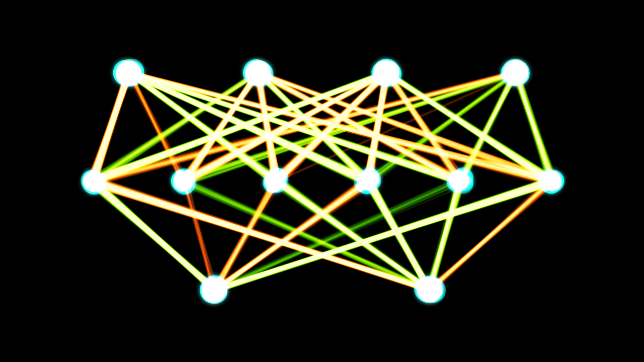
Neural networks have emerged as one of the most powerful and widely-used tools in the field of artificial intelligence and machine learning. These bio-inspired models are capable of learning complex patterns and relationships from data, enabling breakthroughs in areas like computer vision, natural language processing, and robotics.
However, designing and training effective neural networks is far from a trivial task. Two of the most crucial considerations are determining the optimal number of neurons in each layer, and understanding the process of forward propagation that allows networks to generate outputs from inputs.
In this article, we‘ll take a deep dive into these twin pillars of neural network architecture and operation. We‘ll explore cutting-edge techniques for estimating neuron counts, walk through concrete examples of forward propagation in action, and highlight key challenges and opportunities for future research. By the end, you‘ll have a newfound appreciation for the art and science of neural networks, and be well-equipped to start building your own state-of-the-art models.
The Quest for the Perfect Number of Neurons
One of the first steps in designing a neural network is deciding how many neurons to include in each layer. This is a critical decision, as the number of neurons directly impacts the network‘s capacity to learn and generalize from data.
Too few neurons, and the network may underfit, failing to capture the underlying patterns in the training data. Too many neurons, and the network may overfit, essentially memorizing the training examples instead of learning general rules that can be applied to new data.
Traditionally, the process of selecting the right number of neurons has been largely a matter of trial and error, guided by heuristics and experience. However, in recent years, there has been a surge of interest in more principled and automated approaches to this problem.
One promising direction is the field of neural architecture search (NAS), which seeks to automatically discover optimal network architectures through techniques like reinforcement learning and evolutionary algorithms. For example, a 2019 paper by researchers at Google Brain and Stanford University proposed a NAS algorithm called DARTS (Differentiable Architecture Search) that can efficiently search for high-performing architectures using gradient-based optimization [1].
Another approach is to use meta-learning, or "learning to learn," to adaptively adjust the number of neurons based on the characteristics of the data and the task at hand. A 2020 study by researchers at MIT and IBM proposed a meta-learning framework called AdaNet that can automatically adapt the architecture of a neural network to the complexity of the problem [2].
While these advanced techniques are still an active area of research, there are also some general guidelines that practitioners can follow when estimating neuron counts:
- Start with a relatively small number of neurons and gradually increase until performance plateaus
- Use cross-validation to assess generalization performance and detect overfitting
- Consider pruning techniques to remove redundant or low-importance neurons
- Look to successful architectures in the literature as a starting point
Ultimately, the optimal number of neurons will depend on the specific problem and dataset, but by combining domain knowledge with systematic experimentation and advanced search techniques, we can zero in on architectures that strike the right balance between complexity and generalization.
Forward Propagation: From Inputs to Outputs
Once we‘ve settled on a network architecture, the next step is to actually use it to make predictions. This is where forward propagation comes in – the process by which input data is transformed into output predictions as it flows through the layers of the network.
At a high level, forward propagation involves a series of matrix multiplications and element-wise nonlinear transformations. Let‘s walk through a concrete example to see how it works in practice.
Suppose we have a simple feedforward network with an input layer of 3 neurons, a hidden layer of 4 neurons, and an output layer of 2 neurons. We‘ll use the sigmoid activation function in the hidden and output layers.
Given an input vector x = [1, 2, 3], the first step is to multiply it by the weights of the connections between the input and hidden layers, which we‘ll call W1:
W1 = [[-0.5, 0.3, 0.1],
      [0.2, -0.4, 0.8],
      [0.7, 0.2, -0.6],
      [-0.1, 0.9, 0.4]]
Multiplying x by W1 gives us the weighted sum of the inputs to each hidden neuron:
z1 = [[-0.5, 0.3, 0.1] · [1, 2, 3],
      [0.2, -0.4, 0.8] · [1, 2, 3],
      [0.7, 0.2, -0.6] · [1, 2, 3],
      [-0.1, 0.9, 0.4] · [1, 2, 3]]
    = [-0.2, 0.8, 0.3, 2.3]
We then apply the sigmoid activation function element-wise to z1 to get the activations of the hidden neurons:
a1 = sigmoid(z1)
    = [0.45, 0.69, 0.57, 0.91]
The same process is repeated to propagate the activations of the hidden neurons to the output layer. If the weights of the connections between the hidden and output layers are:
W2 = [[0.1, -0.3, 0.5, 0.2],
      [-0.4, 0.6, -0.1, 0.8]]
Then the weighted sum of the inputs to the output neurons is:
z2 = [[0.1, -0.3, 0.5, 0.2] · [0.45, 0.69, 0.57, 0.91],
      [-0.4, 0.6, -0.1, 0.8] · [0.45, 0.69, 0.57, 0.91]]
    = [0.53, 1.01]
And the final output activations after applying the sigmoid function are:
a2 = sigmoid(z2)
    = [0.63, 0.73]
So given an input of [1, 2, 3], our simple network outputs [0.63, 0.73].
Of course, this is just a toy example – real-world neural networks can have millions or even billions of parameters, and use more complex activation functions like ReLU and softmax. But the basic principles of forward propagation remain the same.
Implementing forward propagation in code is relatively straightforward, especially with the help of deep learning frameworks like TensorFlow and PyTorch that handle much of the low-level math behind the scenes. Here‘s a simple example in Python using NumPy:
import numpy as np

def sigmoid(x):
    return 1 / (1 + np.exp(-x))

# Input vector
x = np.array([1, 2, 3])

# Hidden layer weights and biases
W1 = np.array([[-0.5, 0.3, 0.1],
               [0.2, -0.4, 0.8],
               [0.7, 0.2, -0.6],
               [-0.1, 0.9, 0.4]])
b1 = np.array([0.1, -0.2, 0.3, -0.4])

# Output layer weights and biases
W2 = np.array([[0.1, -0.3, 0.5, 0.2],
               [-0.4, 0.6, -0.1, 0.8]])
b2 = np.array([0.2, -0.3])

# Forward propagation
z1 = np.dot(W1, x) + b1
a1 = sigmoid(z1)
z2 = np.dot(W2, a1) + b2
a2 = sigmoid(z2)

print(a2)
This code defines the network parameters (weights and biases) as NumPy arrays, then performs the forward propagation step-by-step, printing the final output activations.
While this example uses a simple sigmoid activation function, in practice, most modern neural networks use piecewise linear functions like ReLU (Rectified Linear Unit) that are more computationally efficient and easier to optimize. The ReLU function is defined as:
f(x) = max(0, x)That is, it returns 0 for negative inputs and the input itself for positive inputs. This simple function has been shown to significantly speed up training and improve generalization performance compared to sigmoid and tanh activations [3].
Activation functions play a crucial role in allowing neural networks to learn nonlinear relationships between inputs and outputs. Without them, even a network with many layers would be equivalent to a linear regression model, severely limiting its representational power.
The choice of activation function can also have a significant impact on the network‘s performance and training dynamics. For example, sigmoid activations are prone to the "vanishing gradient" problem, where gradients become very small as they are backpropagated through the network, making it difficult to train deep networks. ReLU activations, on the other hand, do not suffer from this problem, as their gradients are either 0 or 1.
In addition to ReLU, there are many other activation functions used in neural networks, including:
- Leaky ReLU: A variant of ReLU that allows small negative values to pass through, helping to alleviate the "dying ReLU" problem where neurons get stuck in a permanently inactive state.
- ELU (Exponential Linear Unit): Another ReLU variant that has negative saturation for negative inputs, which can help speed up learning and improve generalization.
- Swish: A recently proposed activation function that combines the properties of ReLU and sigmoid, defined as
f(x) = x * sigmoid(x). Swish has been shown to outperform ReLU on a number of benchmarks [4].
The choice of activation function is just one of many hyperparameters that must be tuned when designing and training neural networks. Others include the learning rate, batch size, regularization strength, and network depth and width.
While there are some general best practices and rules of thumb, finding the optimal hyperparameter settings often requires a combination of domain expertise, empirical experimentation, and automated search techniques like grid search, random search, and Bayesian optimization.
Applications and Future Directions
Forward propagation is the workhorse of neural network inference, enabling these models to tackle an ever-expanding range of applications across domains. Some of the most prominent examples include:
-
Computer Vision: Convolutional neural networks (CNNs) have revolutionized the field of computer vision, achieving human-level or even superhuman performance on tasks like image classification, object detection, and semantic segmentation. Forward propagation in CNNs involves convolving the input image with learned filters to extract hierarchical features at different scales and locations.
-
Natural Language Processing: Recurrent neural networks (RNNs) and transformer models have become the go-to tools for natural language tasks like language modeling, machine translation, and sentiment analysis. Forward propagation in these models involves processing sequences of words or characters one step at a time, using techniques like LSTMs (Long Short-Term Memory) and attention mechanisms to capture long-range dependencies.
-
Reinforcement Learning: Deep reinforcement learning (RL) has achieved remarkable successes in domains like game-playing and robotics, learning complex policies through trial-and-error interaction with an environment. Forward propagation in deep RL involves using a neural network to approximate the value function or policy, which maps states to actions or estimates of future reward.
While neural networks have come a long way in recent years, there are still many open challenges and opportunities for future research. Some of the key frontiers include:
-
Interpretability and Explainability: As neural networks become more complex and powerful, there is a growing need for techniques that can help us understand and interpret their predictions. This is especially important in high-stakes domains like healthcare and finance, where decisions made by AI systems can have significant consequences.
-
Robustness and Security: Neural networks are known to be vulnerable to adversarial examples – inputs that are specifically crafted to fool the model into making incorrect predictions. Developing methods for training robust and secure networks that can withstand these attacks is an active area of research.
-
Transfer and Few-Shot Learning: While deep learning has achieved impressive results on many benchmarks, it typically requires large amounts of labeled training data to work well. Techniques for transferring knowledge between tasks and learning from few examples could help make these models more practical and scalable.
-
Unsupervised and Self-Supervised Learning: Most successful applications of deep learning to date have relied on supervised learning, where the model is trained on a large dataset of labeled examples. However, labeling data is often expensive and time-consuming. Unsupervised and self-supervised learning methods that can learn useful representations from unlabeled data could help unlock the full potential of deep learning.
Conclusion
Estimating the optimal number of neurons and understanding forward propagation are two essential skills for anyone working with neural networks. By mastering these concepts, you can design and train models that are both effective and efficient, and tackle a wide range of real-world problems.
Of course, this is just the beginning of the journey. As the field of deep learning continues to evolve at a rapid pace, staying up-to-date with the latest techniques and best practices is an ongoing challenge. But with a solid foundation in the fundamentals, and a willingness to experiment and innovate, the possibilities are endless.
So go forth and build some amazing neural networks! The world is waiting to see what you‘ll create.


