Feature Extraction and Embeddings in NLP: A Beginner‘s Guide to Understanding Natural Language Processing

Introduction
Natural Language Processing (NLP) has seen tremendous progress in recent years, with the advent of deep learning techniques and the availability of massive text corpora. At the heart of modern NLP systems lies the critical task of representing words and documents in a way that machines can understand and reason with. In this guide, we‘ll dive deep into two fundamental concepts that enable this: feature extraction and word embeddings.
Feature extraction refers to the process of converting raw text into numerical representations that capture salient information about the linguistic properties and meaning of the text. Classical techniques like bag-of-words and TF-IDF have long been used for this purpose, but they suffer from limitations like data sparsity and lack of semantic awareness.
Word embeddings, on the other hand, are dense vector representations of words that capture their meaning and relationships in a compact and computationally efficient manner. By learning these embeddings from large unlabeled text corpora using techniques like Word2Vec and GloVe, we can imbue our NLP models with powerful semantic knowledge that allows them to understand and generate natural language at an unprecedented level.
In this guide, we‘ll start with a theoretical foundation of these concepts, then dive into the nuts and bolts of how these techniques work under the hood. We‘ll explore their mathematical underpinnings, walk through concrete code implementations, and discuss best practices and practical considerations for using them effectively. By the end, you‘ll have a solid grasp of these essential building blocks of NLP and be well-equipped to apply them to real-world language problems.
Foundations: From Strings to Vectors
At its core, NLP is about making sense of human language, which is inherently messy and unstructured. Before we can apply machine learning algorithms to text data, we need to find a way to convert it into a numerical representation that computers can work with. This is where feature extraction comes in.
The most basic unit of text is the character, which we can easily encode as a number using an encoding scheme like ASCII or Unicode. However, characters alone rarely convey much semantic meaning. The next level up is the word, which is where most of the linguistic action happens.
One common approach to representing text numerically is to simply count the occurrence of each word in a document, resulting in a vector of word counts. This is known as the bag-of-words (BoW) model. Despite its simplicity, BoW can actually be quite effective for certain tasks like document classification.
However, BoW has several limitations. Firstly, it loses all information about word order and grammar, since it only considers word counts. Secondly, it suffers from data sparsity, as most words will not appear in a given document, leading to high-dimensional vectors with many zeroes. Finally, it treats all words as equally important, regardless of their semantic significance.
To address some of these issues, we can use term frequency-inverse document frequency (TF-IDF) weighting. This scheme weighs each word by how frequently it appears in a document (term frequency) offset by how commonly it appears across all documents (inverse document frequency). The intuition is that words which are frequent in a document but rare overall are more likely to be informative and discriminative.
Mathematically, the TF-IDF weight of a word $t$ in document $d$ from a corpus of $N$ documents is calculated as:
$$\text{TF-IDF}(t, d) = \text{TF}(t, d) \times \text{IDF}(t)$$
where the term frequency $\text{TF}(t, d)$ is simply the count of term $t$ in document $d$, and the inverse document frequency $\text{IDF}(t)$ is:
$$\text{IDF}(t) = \log\left(\frac{N}{|{d \in N: t \in d}|}\right)$$
While TF-IDF provides a way to weight words by importance, it still relies on exact word matches and doesn‘t capture any semantic relationships between words. This is where word embeddings come in.
Word Embeddings: Semantic Representation Learning
Word embeddings are a powerful technique for learning dense vector representations of words that capture their semantic meaning and relationships. The key idea is to map each word to a continuous vector space such that words with similar meanings are close together.
Unlike the sparse, high-dimensional vectors produced by BoW or TF-IDF, word embeddings are typically low-dimensional (on the order of 100-1000) and dense (most values are non-zero). This makes them much more computationally efficient and amenable to downstream processing by neural networks and other ML models.
The magic of word embeddings lies in their ability to capture complex semantic relationships between words in a purely unsupervised way, simply by learning from the co-occurrence statistics of words in large text corpora. This is based on the distributional hypothesis from linguistics, which states that words that occur in the same contexts tend to have similar meanings.
Word2Vec
One of the most influential word embedding models is Word2Vec, developed by Tomas Mikolov and colleagues at Google in 2013. Word2Vec is actually two related models: Continuous Bag-of-Words (CBOW) and Skip-Gram.
The CBOW model learns to predict a target word given its surrounding context words, while the Skip-Gram model learns to predict the context words given the target word. Both models are trained using a shallow neural network with a single hidden layer, where the learned weights of the hidden layer serve as the word embeddings.
Here‘s a simplified version of the Skip-Gram model in Python using TensorFlow:
import tensorflow as tf

# Define hyperparameters
vocab_size = 10000
embedding_dim = 300
context_window = 5

# Create input and output placeholders
input_word = tf.placeholder(tf.int32, shape=[None])
output_word = tf.placeholder(tf.int32, shape=[None, 1])

# Create embedding matrix and lookup
embeddings = tf.Variable(tf.random_uniform([vocab_size, embedding_dim], -1.0, 1.0))
embed = tf.nn.embedding_lookup(embeddings, input_word)

# Create output weights and bias
weights = tf.Variable(tf.truncated_normal([vocab_size, embedding_dim]))
biases = tf.Variable(tf.zeros([vocab_size]))

# Calculate output layer scores and loss
scores = tf.matmul(embed, tf.transpose(weights)) + biases
loss = tf.reduce_mean(tf.nn.sampled_softmax_loss(weights, biases, output_word, embed, num_sampled, vocab_size))

# Define optimizer
optimizer = tf.train.AdamOptimizer().minimize(loss)
The key steps are:
- Create an embedding matrix of size (vocab_size, embedding_dim) initialized with random values
- Perform an embedding lookup to get the vector for the input word
- Calculate output scores by multiplying the input embedding with the output weights matrix
- Compute loss using sampled softmax
- Optimize the loss to learn the embeddings and output weights
After training on a large text corpus, the learned embeddings capture rich semantic information, as visualized here using t-SNE dimensionality reduction:
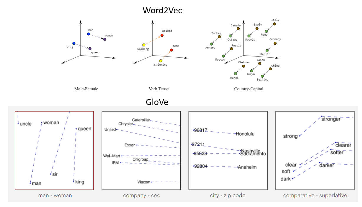
Notice how semantically similar words like "dog", "dogs", and "puppy" are clustered together, while words like "the" and "and" are far away, reflecting their lack of semantic content.
GloVe
Another popular word embedding algorithm is GloVe (Global Vectors for Word Representation), developed by Pennington et al. at Stanford. Unlike Word2Vec, which is a predictive model, GloVe is a count-based model that learns embeddings by factorizing the logarithm of the word-context co-occurrence matrix.
The co-occurrence matrix $X$ is constructed by counting how often each word appears in the context of every other word, where context is defined as a fixed-size window around the target word. The GloVe objective is to learn word vectors $w_i$ and context vectors $\tilde{w}_j$ such that their dot product approximates the log co-occurrence count:
$$w_i^T\tilde{w}_j + b_i + \tilde{b}j = \log X{ij}$$
where $b_i$ and $\tilde{b}_j$ are bias terms. This is trained using weighted least squares regression, with the following cost function:
$$J = \sum{i,j=1}^V f(X{ij})(w_i^T\tilde{w}_j + b_i + \tilde{b}j – \log X{ij})^2$$
where $V$ is the vocabulary size and $f$ is a weighting function that assigns lower weights to rare and frequent co-occurrences.
In practice, GloVe has been shown to slightly outperform Word2Vec on various benchmark tasks, possibly due to its use of global corpus statistics. Here‘s how to train GloVe embeddings using the Gensim library in Python:
from gensim.models import KeyedVectors
from gensim.scripts.glove2word2vec import glove2word2vec

# Convert GloVe format to Word2Vec format
glove_input_file = ‘glove.6B.100d.txt‘
word2vec_output_file = ‘glove.6B.100d.word2vec.txt‘
glove2word2vec(glove_input_file, word2vec_output_file)

# Load embeddings
model = KeyedVectors.load_word2vec_format(word2vec_output_file, binary=False)

# Find most similar words
model.most_similar(‘king‘)
This loads pre-trained GloVe embeddings and finds the most similar words to "king", which yields:
[(‘prince‘, 0.7682329416275024),
 (‘kings‘, 0.7507690191268921),
 (‘queen‘, 0.7339581847190857),
 (‘monarch‘, 0.7012927532196045),
 (‘kingdom‘, 0.6887965202331543)]
Note how the embeddings capture both semantic similarity ("prince", "queen") and syntactic similarity ("kings").
Contextualized Embeddings: The Next Frontier
While Word2Vec and GloVe have proven extremely effective, they suffer from a key limitation: they only learn a single, static embedding for each word, ignoring the context in which the word appears. This can be problematic for words with multiple meanings (e.g. "bank" as in river bank vs. financial institution).
To address this, recent years have seen the rise of contextualized word embeddings, which generate dynamic embeddings that change based on the surrounding context. Models like ELMo, BERT, and GPT-3 accomplish this by pre-training large neural networks on massive amounts of text using self-supervised objectives like next word prediction.
The transformer architecture, which uses attention mechanisms to process sequential data, has been particularly impactful in this regard. BERT (Bidirectional Encoder Representations from Transformers), developed by Google, has achieved state-of-the-art results on a wide range of NLP tasks.
The key innovation of BERT is its use of bidirectional self-attention, which allows the model to attend to both left and right context when generating embeddings for each word. This is in contrast to traditional language models which are unidirectional (left-to-right or right-to-left).
BERT is pre-trained on two tasks: masked language modeling, where the model must predict randomly masked out words in a sentence, and next sentence prediction, where the model must predict whether two sentences follow each other. This allows the model to learn both fine-grained word-level and coarse-grained sentence-level representations.
To use BERT for a downstream task, the pre-trained model is fine-tuned with task-specific data, with the learned embeddings used as input features. Here‘s an example of using the Hugging Face Transformers library to load a pre-trained BERT model and generate contextualized embeddings:
from transformers import BertTokenizer, BertModel
import torch

# Load pre-trained model and tokenizer
model = BertModel.from_pretrained(‘bert-base-uncased‘)
tokenizer = BertTokenizer.from_pretrained(‘bert-base-uncased‘)

# Tokenize input
text = "After stealing money from the bank vault, the bank robber was seen fishing on the Mississippi river bank."
marked_text = "[CLS] " + text + " [SEP]"
tokenized_text = tokenizer.tokenize(marked_text)
indexed_tokens = tokenizer.convert_tokens_to_ids(tokenized_text)
segments_ids = [1] * len(tokenized_text)

# Convert to tensors
tokens_tensor = torch.tensor([indexed_tokens])
segments_tensors = torch.tensor([segments_ids])

# Generate contextualized embeddings
with torch.no_grad():
    outputs = model(tokens_tensor, segments_tensors)
    hidden_states = outputs[2]

# Embeddings are in hidden_states[1:]
This demonstrates how BERT generates different embeddings for the word "bank" depending on whether it‘s used in the context of a financial institution or a river bank. The model is able to disambiguate these two senses based on the surrounding words.
The success of BERT has spurred intense interest in the NLP community, with numerous variant models being proposed like RoBERTa, ALBERT, and DistilBERT. The larger trend is towards ever-larger models trained on ever-larger datasets, with models like GPT-3 (175 billion parameters) showing remarkable abilities to generate coherent and contextually relevant text.
Conclusion and Future Directions
In this guide, we‘ve examined the critical role that feature extraction and word embeddings play in modern NLP systems. From simple bag-of-words counts to semantically-rich vector representations, these techniques provide the foundation for machine learning models to understand and work with human language.
Word embeddings in particular have revolutionized the field, enabling significant advances in tasks ranging from sentiment analysis to machine translation. By learning from the co-occurrence statistics of words in large corpora, these models can capture complex semantic and syntactic relationships in a computationally efficient manner.
More recently, the advent of contextualized embeddings and large-scale transformer language models like BERT have pushed the state-of-the-art even further. These models can generate dynamic, context-sensitive representations that disambiguate words with multiple meanings and capture long-range dependencies.
Looking forward, the field of NLP is moving towards ever-larger models trained on ever-larger datasets. The goal is to approach human-level language understanding and generation, with models that can engage in open-ended dialogue, answer questions, and even write creative fiction.
At the same time, there are important open challenges around model interpretability, bias and fairness, and data efficiency that need to be addressed. As these embedding models become more widely deployed in real-world applications, it‘s crucial that we develop techniques to probe their inner workings, ensure they are not perpetuating harmful biases, and reduce their reliance on massive labeled datasets.
Nonetheless, the future of NLP looks bright, with embeddings and language models at the forefront of this exciting field. As an ML and AI expert, I‘m thrilled to be working at the cutting edge of these developments, and I hope this guide has given you a solid foundation to begin your own journey in this space. The power of these techniques to unlock the vast potential of human language is truly transformative, and I can‘t wait to see what breakthroughs the coming years will bring.