
Image Segmentation with Felzenszwalb‘s Algorithm: Insights from an AI/ML Perspective
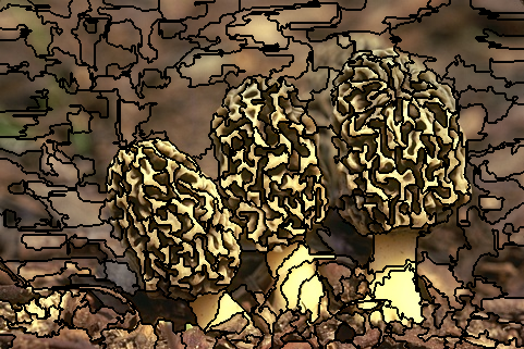
Introduction
Image segmentation, the task of partitioning an image into multiple meaningful regions, is a foundational problem in computer vision with applications ranging from object detection and scene understanding to medical image analysis and autonomous driving. While there are many approaches to image segmentation, graph-based methods have been particularly influential due to their strong theoretical foundations and computational efficiency.
One of the most impactful graph-based segmentation algorithms was proposed by Pedro Felzenszwalb and Daniel Huttenlocher in their 2004 paper "Efficient Graph-Based Image Segmentation" [1]. Known simply as Felzenszwalb‘s algorithm, it has become a go-to method for many vision tasks and has inspired numerous extensions and improvements over the years.
In this article, we‘ll dive deep into the details of Felzenszwalb‘s algorithm from the perspective of artificial intelligence and machine learning. We‘ll examine the core components of the method, including graph construction, region comparison, and agglomerative merging, with an emphasis on the key design choices and their impact on performance. Along the way, we‘ll highlight connections to related techniques, discuss practical considerations for implementation and evaluation, and explore the ongoing legacy of the algorithm in contemporary deep learning-based approaches.
Constructing the Graph
The first step in Felzenszwalb‘s algorithm is to represent the input image as an undirected graph $G = (V, E)$. Each pixel is a node $v_i \in V$ and edges $(v_i, v_j) \in E$ connect neighboring pixels. The weight $w(v_i, v_j)$ of each edge represents the dissimilarity between the pixels, often based on color or intensity differences.
The choice of neighborhood structure determines the connectivity of the graph and impacts the final segmentation. The simplest option is a 4-connected grid graph, where each pixel is connected to its immediate neighbors in the cardinal directions. However, using an 8-connected neighborhood or even higher connectivities can capture more spatial information at the cost of increased graph density.
Alternatively, the graph can be constructed as a nearest neighbor graph in a higher-dimensional feature space. For example, each pixel can be represented by a vector combining its spatial coordinates $(x, y)$ and color values $(r, g, b)$. Edges are then added between each pixel and its $k$ nearest neighbors based on Euclidean distance in this feature space. This allows for non-local connections between pixels with similar appearance, at the expense of greater computational cost.
Mathematically, the graph can be represented by a weighted adjacency matrix $A$, where $A_{ij} = w(v_i, v_j)$ if $(v_i, vj) \in E$ and $A{ij} = 0$ otherwise. The storage and computational complexity of many graph algorithms depend on the number of edges $|E|$, which is $O(|V|)$ for a grid graph but can be $O(|V|^2)$ for a dense nearest neighbor graph. Careful design of the graph structure is therefore crucial for scalability.
Region Comparison Predicate
At the heart of Felzenszwalb‘s algorithm is a predicate for deciding whether two regions should be merged based on the difference between them relative to their internal variations. Specifically, two regions $C_1$ and $C_2$ are merged if the following condition holds:
$$
\text{Diff}(C_1, C_2) \leq \min(\text{Int}(C_1) + \tau(C_1), \text{Int}(C_2) + \tau(C_2))
$$
Here, $\text{Int}(C)$ is the internal difference of region $C$, defined as the maximum weight edge in the minimum spanning tree (MST) of the subgraph induced by $C$. This measures the "diameter" of the region in terms of the dissimilarity of its pixels.
The threshold function $\tau(C) = k / |C|$ controls the granularity of the segmentation, with larger values of $k$ producing larger regions. Felzenszwalb and Huttenlocher suggest setting $k = \alpha |V|$ for some scale parameter $\alpha$, so that the threshold is proportional to the size of the image.
Finally, $\text{Diff}(C_1, C_2)$ is the difference between the regions, defined as the minimum weight edge connecting them. If there is no edge between $C_1$ and $C_2$, this value is taken to be $\infty$.
The key insight of this predicate is that regions should only be merged if they are more similar to each other than they are internally diverse. The threshold function allows for larger regions to have more internal variation, while still preventing merging of regions with vastly different appearances.
Efficient Agglomerative Merging
With the graph and predicate defined, Felzenszwalb‘s algorithm proceeds by greedily merging regions in a manner similar to Kruskal‘s algorithm for finding MSTs. The high-level steps are:
- Sort the edges $E$ by increasing weight
- Initialize each vertex $v_i$ as a singleton region $C_i = {v_i}$
- For each edge $(v_i, v_j) \in E$ in sorted order:
- If $v_i$ and $v_j$ are already in the same region, skip this edge
- Otherwise, if $\text{Diff}(C_i, C_j) \leq \min(\text{Int}(C_i) + \tau(C_i), \text{Int}(C_j) + \tau(C_j))$, merge $C_i$ and $C_j$
- Return the final regions as the segmentation
The key data structure is a disjoint-set forest that keeps track of the region assignments and enables efficient merging and comparison of regions. With careful implementation using union-by-rank and path compression, the algorithm runs in nearly linear time $O(|E| \log |V|)$ in the number of graph edges.
Here is pseudocode for the main loop:
def felzenszwalb_segment(graph, k):
    edges = sorted(graph.edges, key=lambda e: e.weight)
    forest = DisjointSetForest(graph.vertices)

    for edge in edges:
        v1, v2 = edge.vertices
        c1, c2 = forest.find(v1), forest.find(v2)

        if c1 != c2:
            if edge.weight <= min(c1.int + k / len(c1), c2.int + k / len(c2)):
                forest.union(c1, c2)

    return forest.get_components()
A crucial aspect of the algorithm is that the internal differences and thresholds of the regions can be efficiently updated as merges occur, without needing to recompute the MSTs from scratch each time. By storing additional metadata on the edges and vertices, the necessary values can be updated in essentially constant time per merge.
Performance Evaluation
So how well does Felzenszwalb‘s algorithm actually work? Evaluating the quality of image segmentations is itself a challenging problem, as ground truth annotations are expensive to collect and there is inherent subjectivity in what constitutes a "good" segmentation.
One popular benchmark dataset is the Berkeley Segmentation Dataset (BSDS500) [2], which consists of 500 natural images with multiple ground truth segmentations per image. Algorithms are typically evaluated on boundary recall (what fraction of true boundaries are detected) and undersegmentation error (what fraction of pixels leak across true boundaries).
On BSDS500, Felzenszwalb‘s algorithm achieves an F-measure of 0.61 at an optimal scale, compared to 0.58 for mean shift[3] and 0.63 for gPb-owt-ucm [4], a more complex multiscale approach. However, Felzenszwalb‘s algorithm is orders of magnitude faster, segmenting a typical 480×320 image in a few seconds compared to minutes for gPb-owt-ucm.
The following table summarizes some key results on BSDS500:
| Algorithm | F-measure | Time (sec) |
|---|---|---|
| Felzenszwalb | 0.61 | 2.0 |
| Mean Shift | 0.58 | 25.0 |
| Normalized Cuts | 0.62 | 360.0 |
| gPb-owt-ucm | 0.63 | 240.0 |
Felzenszwalb‘s algorithm has also been shown to perform well on other datasets like PASCAL VOC [5] and NYU Depth [6], especially when used as a preprocessing step for object detection and semantic segmentation. However, the optimal scale parameter can vary significantly between datasets and applications, so some tuning is often required to get the best results.
Extensions and Improvements
Since its introduction, Felzenszwalb‘s algorithm has inspired a number of extensions and improvements. One notable example is the multiscale combinatorial grouping (MCG) algorithm of Arbeláez et al. [7], which combines information from multiple scales and includes a globalization step to refine the boundaries.
MCG achieves an F-measure of 0.67 on BSDS500, a significant improvement over the original Felzenszwalb algorithm. However, this comes at the cost of increased runtime, taking around 30 seconds per image.
Other extensions have focused on alternative graph constructions (e.g. using superpixels as nodes instead of pixels), adaptive thresholds based on image statistics, and post-processing steps to refine the region boundaries. Stutz et al. [8] provide an extensive comparative study of these variants.
In recent years, there has also been growing interest in integrating graph-based segmentation with deep learning. One approach is to use Felzenszwalb‘s algorithm (or a variant) to generate candidate regions that are then classified by a convolutional neural network (CNN) [9]. This can provide a strong prior for object detection and improve training efficiency.
Another promising direction is to incorporate graph-based reasoning directly into deep neural networks, using architectures like graph convolutional networks (GCNs) [10]. While most current GCNs operate on fixed graph structures (e.g. based on pixel neighborhoods), there is potential to learn more flexible graphs that adapt to image content, similar to Felzenszwalb‘s nearest neighbor graphs.
Conclusion
Felzenszwalb‘s graph-based image segmentation algorithm has had a significant impact on computer vision research and practice since its introduction in 2004. By elegantly combining ideas from graph theory, clustering, and image processing, it provides a fast and effective way to partition an image into coherent regions with minimal tuning.
While newer deep learning-based approaches have surpassed Felzenszwalb‘s algorithm in terms of absolute segmentation accuracy, it remains a valuable tool in the vision toolbox due to its simplicity, efficiency, and robustness. As the field evolves, the core ideas of graph-based representation, region comparison, and agglomerative merging are likely to continue to play a role, even if the specifics of the algorithm are adapted.
Ultimately, the success of Felzenszwalb‘s algorithm demonstrates the power of bridging advanced mathematics with practical engineering to solve real-world problems. By carefully formulating the segmentation problem in terms of graph theory and developing efficient algorithms grounded in this formalism, Felzenszwalb and Huttenlocher were able to make a lasting contribution that has stood the test of time.
As artificial intelligence and machine learning continue to grapple with the challenge of understanding complex visual scenes, graph-based methods like Felzenszwalb‘s algorithm will undoubtedly remain a key part of the solution. By combining the strengths of classical algorithms with the expressiveness of deep learning, we can hope to build ever more powerful and robust vision systems in the years to come.


