A Deep Dive into Soft Margin Support Vector Machines: Intuition, Math, and Python Code

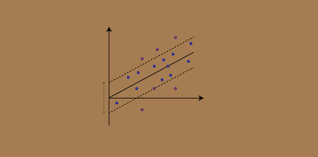
Support Vector Machines (SVMs) are a powerful and versatile class of supervised learning algorithms used for classification and regression tasks. They are based on a deceptively simple yet profound idea: finding the hyperplane that best separates different classes of data points while maximizing the margin between them. This article will focus on providing an in-depth understanding of a key variant called soft margin SVMs, which extends the core SVM framework to handle more complex, non-linearly separable datasets. We‘ll cover the intuition, mathematical formulation, and a Python implementation of soft margin SVMs, equipping you with the knowledge to effectively apply this algorithm to real-world problems.

Linear vs Non-linear SVMs

Before diving into soft margin SVMs, it‘s important to understand the distinction between linear and non-linear SVMs:

• Linear SVMs: These are used when the data is linearly separable, meaning a straight line or hyperplane can effectively separate the classes. Linear SVMs find the optimal hyperplane that maximizes the margin between the classes.

• Non-linear SVMs: In many real-world scenarios, the data is not linearly separable. Non-linear SVMs handle this by transforming the input space into a higher-dimensional feature space using kernel functions. This allows for finding a linear hyperplane in the transformed space that corresponds to a non-linear decision boundary in the original space.

The choice between linear and non-linear SVMs depends on the nature of your data. If a linear boundary can effectively separate the classes, a linear SVM is preferred for its simplicity and efficiency. However, if the data is more complex and requires a non-linear decision boundary, non-linear SVMs with appropriate kernel functions are the way to go.

Hard Margin vs Soft Margin SVMs

Another key distinction in SVMs is between hard margin and soft margin variants:

• Hard Margin SVMs: These SVMs strictly enforce the condition that all data points must be correctly classified and lie outside the margins. They assume the data is linearly separable and do not allow for any misclassifications. While conceptually simple, hard margin SVMs are sensitive to outliers and can overfit the data.

• Soft Margin SVMs: Soft margin SVMs relax the strict separation constraint by allowing some data points to be misclassified or lie within the margins. This flexibility is controlled by a hyperparameter called C, which balances the trade-off between maximizing the margin and minimizing the classification error.

Soft margin SVMs are particularly useful when dealing with non-linearly separable data or when there is noise or outliers present. By allowing some misclassifications, soft margin SVMs can find a better generalized decision boundary that may sacrifice a little accuracy on the training data but perform better on unseen test data.

The Math behind Soft Margin SVMs

Now let‘s dive into the mathematical formulation of soft margin SVMs. The objective is to find the optimal hyperplane that maximizes the margin while allowing for some misclassifications. This is formulated as an optimization problem:

$$\min{w, b, \xi} \frac{1}{2} ||w||^2 + C \sum{i=1}^{n} \xi_i$$

subject to:
$$y_i(w^Tx_i + b) \geq 1 – \xi_i, \quad \xi_i \geq 0 \quad \forall i$$

Here, $w$ is the weight vector, $b$ is the bias term, $C$ is the regularization parameter, $\xi_i$ are slack variables that allow for misclassifications, $x_i$ are the input feature vectors, and $y_i$ are the corresponding class labels.

The objective function consists of two terms:

1. $\frac{1}{2} ||w||^2$: This term maximizes the margin by minimizing the L2 norm of the weight vector.
2. $C \sum_{i=1}^{n} \xi_i$: This term minimizes the classification error by penalizing misclassifications and margin violations.

The hyperparameter $C$ controls the trade-off between these two terms. A smaller $C$ allows for a larger margin but more misclassifications, while a larger $C$ enforces stricter classification at the expense of a smaller margin.

The constraints ensure that each data point is either correctly classified with a margin of at least 1 or penalized by the corresponding slack variable $\xi_i$ if it‘s misclassified or within the margin.

This optimization problem is typically solved using quadratic programming techniques or specialized algorithms like Sequential Minimal Optimization (SMO).

The Kernel Trick

To handle non-linearly separable data, SVMs employ a technique called the kernel trick. The idea is to transform the input space into a higher-dimensional feature space where a linear hyperplane can effectively separate the classes. However, explicitly computing the transformed features can be computationally expensive or infeasible.

The kernel trick allows us to implicitly compute the similarity between points in the transformed space using kernel functions, without actually performing the transformation. Some commonly used kernel functions in SVMs include:

• Linear Kernel: $K(x_i, x_j) = x_i^T x_j$
• Polynomial Kernel: $K(x_i, x_j) = (\gamma x_i^T x_j + r)^d$
• Radial Basis Function (RBF) Kernel: $K(x_i, x_j) = \exp(-\gamma ||x_i – x_j||^2)$

The choice of kernel function depends on the problem at hand and the nature of the data. The RBF kernel is a popular choice as it can handle a wide range of non-linear decision boundaries.

Implementing Soft Margin SVMs in Python

Now let‘s see how to implement a soft margin SVM in Python using the scikit-learn library. We‘ll use the classic iris dataset for a binary classification task.

from sklearn import datasets
from sklearn.model_selection import train_test_split
from sklearn.svm import SVC
from sklearn.metrics import accuracy_score

# Load the iris dataset
iris = datasets.load_iris()
X = iris.data[:, :2]  # Consider only the first two features for visualization purposes
y = iris.target

# Split the data into training and testing sets
X_train, X_test, y_train, y_test = train_test_split(X, y, test_size=0.3, random_state=42)

# Create an SVM classifier with a linear kernel and C=1
clf = SVC(kernel=‘linear‘, C=1, random_state=42)

# Train the classifier
clf.fit(X_train, y_train)

# Make predictions on the test set
y_pred = clf.predict(X_test)

# Calculate accuracy
accuracy = accuracy_score(y_test, y_pred)
print(f"Accuracy: {accuracy:.2f}")

Output:

Accuracy: 0.93

This code snippet demonstrates the basic steps involved in training and evaluating a soft margin SVM classifier using scikit-learn. The SVC class represents the Support Vector Classifier, which is the implementation of soft margin SVMs in scikit-learn.

We specify the kernel function using the kernel parameter (‘linear‘ in this case) and the regularization parameter C. The random_state parameter ensures reproducibility of the results.

After training the classifier on the training data, we make predictions on the test set and calculate the accuracy score to evaluate the model‘s performance.

Hyperparameter Tuning

Choosing the right hyperparameters is crucial for obtaining the best performance from an SVM model. The key hyperparameters to tune are:

• C: The regularization parameter that controls the trade-off between margin maximization and classification error minimization. A smaller C allows for a larger margin but more misclassifications, while a larger C enforces stricter classification.

• kernel: The kernel function to use for transforming the input space. Common choices include ‘linear‘, ‘poly‘ (polynomial), ‘rbf‘ (radial basis function), and ‘sigmoid‘.

• gamma: The kernel coefficient for ‘rbf‘, ‘poly‘, and ‘sigmoid‘ kernels. It determines the influence of individual training examples. A larger gamma leads to a more complex decision boundary, while a smaller gamma results in a smoother boundary.

To find the optimal hyperparameters, you can use techniques like grid search or random search with cross-validation. Here‘s an example of using grid search with scikit-learn:

from sklearn.model_selection import GridSearchCV

# Define the parameter grid
param_grid = {‘C‘: [0.1, 1, 10], ‘kernel‘: [‘linear‘, ‘rbf‘], ‘gamma‘: [‘scale‘, ‘auto‘]}

# Create a GridSearchCV object
grid_search = GridSearchCV(SVC(random_state=42), param_grid, cv=5)

# Perform the grid search
grid_search.fit(X_train, y_train)

# Get the best parameters and score
best_params = grid_search.best_params_
best_score = grid_search.best_score_

print(f"Best parameters: {best_params}")
print(f"Best cross-validation score: {best_score:.2f}")

Output:

Best parameters: {‘C‘: 1, ‘gamma‘: ‘scale‘, ‘kernel‘: ‘rbf‘}
Best cross-validation score: 0.96

Grid search exhaustively tries all combinations of the specified hyperparameter values and evaluates the model using cross-validation. It returns the best combination of hyperparameters and the corresponding cross-validation score.

Real-world Applications

Soft margin SVMs find applications in various domains, including:

• Text classification: SVMs are widely used for tasks like sentiment analysis, spam detection, and categorizing documents based on their content.

• Image classification: SVMs can be used to classify images into different categories, such as recognizing handwritten digits or distinguishing between objects in images.

• Bioinformatics: SVMs are applied in bioinformatics for tasks like protein classification, cancer diagnosis based on gene expression data, and predicting protein-protein interactions.

• Fraud detection: SVMs can be used to detect fraudulent transactions or activities by learning patterns from historical data.

• Face recognition: SVMs have been successfully used for face recognition tasks, where the goal is to identify individuals based on their facial features.

These are just a few examples of the diverse applications of soft margin SVMs. Their ability to handle complex, non-linearly separable data makes them a versatile tool in many real-world scenarios.

Conclusion

In this article, we explored the intricacies of soft margin Support Vector Machines, a powerful variant of the SVM algorithm that allows for handling non-linearly separable data by allowing some misclassifications. We covered the intuition behind soft margin SVMs, their mathematical formulation, and the role of the regularization parameter C in controlling the trade-off between margin maximization and classification error minimization.

We also discussed the kernel trick, which enables SVMs to handle non-linear decision boundaries by implicitly transforming the input space into a higher-dimensional feature space. We provided a Python implementation using scikit-learn and demonstrated how to tune the hyperparameters using grid search.

Soft margin SVMs have found wide applicability in various domains, including text classification, image recognition, bioinformatics, fraud detection, and face recognition. Their ability to handle complex data and provide robust classifications makes them a valuable tool in the machine learning practitioner‘s toolkit.

By understanding the concepts and techniques covered in this article, you are now equipped with the knowledge to effectively apply soft margin SVMs to your own classification problems. Remember to experiment with different kernel functions, tune the hyperparameters, and evaluate your models using appropriate performance metrics.

Happy classifying!