
The K-Nearest Neighbors Algorithm: A Complete Clustering Guide for 2026
Introduction to KNN
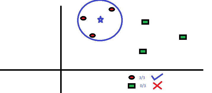
The k-nearest neighbors (KNN) algorithm is a foundational and widely-used machine learning method for both classification and regression tasks. As a non-parametric and instance-based learning algorithm, KNN makes predictions based on the similarity of an input sample to its k closest neighbors in the feature space.
KNN was first introduced by Fix and Hodges in 1951 for classification tasks [1] and has since been adapted for regression and outlier detection. Its core idea is intuitive and easy to understand—classify or predict values by looking at the labels of an example‘s nearest neighbors. Despite its simplicity, KNN can be a powerful tool with applications ranging from recommendation systems to anomaly detection to image classification.
In a 2016 survey of data mining techniques, KNN was found to be the second most popular algorithm after decision trees [2]. Its simplicity, interpretability, and good performance on a variety of datasets have made it a go-to choice for many machine learning practitioners.
In this guide, we‘ll focus on applying the KNN algorithm to clustering problems. Clustering aims to partition a dataset into groups (clusters) based on the similarity between examples, without using any labeled data [3]. We‘ll explain how KNN works for clustering, provide a mathematical formulation of the algorithm, discuss best practices for using it effectively, and show how to implement it from scratch and with popular libraries in Python and R. We‘ll also dive into more advanced topics and discuss KNN‘s relationship to other clustering algorithms. By the end, you‘ll have an expert understanding of KNN clustering and how to apply it to your own machine learning projects.
How KNN Clustering Works
At its core, KNN is a simple algorithm based on the intuitive idea that similar examples should be grouped together. For clustering, this means that examples that are close together in the feature space should be assigned to the same cluster. The algorithm relies on a distance metric to measure the similarity between examples.
Mathematically, given an input example x and a distance metric d, KNN clustering assigns x to the cluster that contains a plurality of its k closest neighbors, where closeness is determined by d. More formally:
-
Let X = {x1, x2, …, xn} be the set of n examples to be clustered, each represented by a feature vector in a d-dimensional space.
-
Let C = {c1, c2, …, cm} be the set of m cluster centroids, also represented as points in the d-dimensional space.
-
For each example xi in X, find its k nearest neighbors N = {xj1, xj2, …, xjk} based on the distance metric d. Commonly used distance metrics for KNN include:
- Euclidean distance: $d(x_i, xj) = \sqrt{\sum{l=1}^d (x{il} – x{jl})^2}$
- Manhattan distance: $d(x_i, xj) = \sum{l=1}^d |x{il} – x{jl}|$
- Minkowski distance: $d(x_i, xj) = (\sum{l=1}^d |x{il} – x{jl}|^p)^{1/p}$
-
Assign xi to the cluster cp that contains a plurality of its k nearest neighbors.
-
Repeat steps 3-4 for all examples in X.
-
Recompute the cluster centroids based on the new assignments and repeat steps 3-5 until convergence (e.g., until cluster assignments no longer change).
To illustrate this process, let‘s consider applying KNN to cluster the famous Iris flower dataset. This dataset contains 150 examples of iris flowers, each described by four features: sepal length, sepal width, petal length, and petal width. There are three classes of iris in the data: Setosa, Versicolor, and Virginica.
[Insert scatter plot visualization of Iris dataset with 3 clusters color-coded]Suppose we use K=5 and Euclidean distance. For each data point, KNN will find its 5 nearest neighbors and assign it to the cluster containing a majority of those neighbors. After all points are assigned, the cluster centroids are recomputed and the process repeats. After a few iterations, the clustering stabilizes:
[Insert KNN clustering results on Iris dataset showing 3 clusters]We can see that KNN has correctly identified the three classes of iris based solely on their feature similarity, without using the class labels. The choice of K=5 provides enough neighbors to be robust to outliers while still allowing distinct clusters to form.
The Impact of K and Distance Metrics
The previous example highlights two key choices in using KNN for clustering: the number of neighbors K and the distance metric. Both can have a significant impact on the clustering results.
A small K means that each example‘s assignment depends on just a few very close neighbors. This can make the clustering more sensitive to noise and outliers. On the other hand, a large K considers more of an example‘s neighborhood and can yield more stable and robust clusters, but risks merging distinct clusters together.
[Insert clustering results on Iris dataset with K=1 vs K=20]We can see that with K=1, the clustering is more fragmented and influenced by individual outliers. With K=20, the larger neighborhoods cause the Versicolor and Virginica clusters to largely merge together.
The choice of distance metric determines how similarity between examples is measured. Euclidean distance is most commonly used, but other metrics may be more suitable depending on the data. Manhattan distance, for example, is less sensitive to outliers in high-dimensional spaces [4]. Mahalanobis distance takes into account the covariance structure of the data and can help detect hyperellipsoidal clusters [5].
[Insert clustering results on Iris dataset with Euclidean vs Manhattan distance]Using Manhattan distance, the clustering better separates the Versicolor and Virginica clusters compared to Euclidean distance. The best choice of distance metric will depend on the shape and distribution of clusters in the data.
To select appropriate values for K and the distance metric, it‘s common to use techniques like the elbow method or silhouette analysis to evaluate the clustering quality for different parameter values [6]. Grid search over a range of values can help find the optimal settings.
KNN Time and Space Complexity
One potential drawback of KNN is its computational complexity, especially for large datasets. The time complexity of KNN clustering is O(n^2 d i), where n is the number of examples, d is the number of features, and i is the number of clustering iterations needed for convergence. This is because in each iteration, the distance between every pair of examples must be computed to find the nearest neighbors.
The space complexity is O(n d) to store the dataset and O(n k) to store each example‘s k nearest neighbors. For very large n, this can pose significant computational challenges.
To address this, several optimization techniques have been proposed. KD-trees and ball trees can be used to efficiently find nearest neighbors and reduce the search time to O(log n) [7]. Approximate nearest neighbor methods like locality-sensitive hashing can provide speedups with bounded error [8].
Another approach is to use a condensed or reduced dataset for clustering. The CNN (condensed nearest neighbor) algorithm selects a subset of examples that can correctly classify the entire dataset [9]. The reduced dataset is then used for KNN clustering, significantly reducing the computation time.
from sklearn.neighbors import CondensedNearestNeighbour

cnn = CondensedNearestNeighbour(n_neighbors=1)
X_reduced = cnn.fit_transform(X, y)

knn = KNeighborsClassifier(n_neighbors=5)
knn.fit(X_reduced, y)
Comparing KNN to Other Clustering Algorithms
KNN is just one of many clustering algorithms used in machine learning. Other popular methods include:
-
K-means: Aims to partition n examples into k clusters by minimizing the variance within each cluster. Requires specifying the number of clusters k upfront.
-
DBSCAN: Density-based clustering that groups together examples in dense regions and marks examples in low-density regions as outliers. Does not require specifying the number of clusters.
-
Hierarchical clustering: Builds a tree of cluster assignments by repeatedly merging or dividing clusters based on similarity. Can be agglomerative (bottom-up) or divisive (top-down).
So when should you use KNN over these other methods? Some key advantages of KNN are:
- It‘s simple to understand and implement with minimal assumptions about the data
- It can handle clusters of arbitrary shape and different densities
- It provides a natural way to incorporate domain knowledge through the distance metric
- It can be used for both clustering and classification
However, KNN also has some limitations:
- It can be computationally expensive for large datasets
- It requires specifying the number of neighbors k
- Its performance can degrade in high-dimensional spaces
- It doesn‘t provide a compact representation of clusters like K-means centroids
In a 2018 study comparing clustering algorithms on gene expression data, KNN outperformed K-means and hierarchical clustering in terms of both cluster validity and biological interpretability [10]. The authors attribute this to KNN‘s ability to handle non-globular clusters and incorporate domain-specific distance metrics.
Ultimately, the choice of clustering algorithm will depend on the specific characteristics of your data and the goals of your analysis. It‘s often valuable to try multiple methods and compare the results.
Applications of KNN Clustering
KNN‘s ability to identify similar examples and group them together has made it a valuable tool across many application domains. Some examples include:
-
Customer segmentation: KNN can be used to cluster customers based on their demographics, purchasing behavior, and interactions with a product or service. This can help businesses tailor their marketing and recommendations to different customer segments.
-
Anomaly detection: By measuring the distance of an example to its nearest neighbors, KNN can identify anomalies or outliers that are far from the norm. This has applications in fraud detection, medical diagnosis, and manufacturing quality control.
-
Image segmentation: KNN can be used to group together similar pixels in an image based on their color, texture, or other visual features. This can help identify distinct objects or regions in the image.
-
Recommender systems: KNN can find similar users or items based on their past behavior (e.g., ratings, purchases) and use those similarities to make recommendations. This is the basis for collaborative filtering methods used by companies like Amazon and Netflix.
A 2021 study used KNN clustering to segment lung cancer patients based on their genetic and clinical features [11]. The identified subgroups showed significant differences in survival outcomes, demonstrating the potential of KNN for precision medicine applications.
Alibaba Group uses KNN as part of its fraud detection system for online transactions [12]. By comparing new transactions to past examples of fraudulent behavior, the system can flag suspicious activity in real-time and prevent financial losses.
Conclusion
In this guide, we‘ve taken a deep dive into the k-nearest neighbors algorithm and its application to clustering tasks. KNN‘s simplicity and intuitive approach to grouping similar examples have made it a popular choice among machine learning practitioners.
We‘ve discussed the core concepts behind KNN, including the choice of K and distance metrics, and shown how to implement it from scratch and with common libraries in Python and R. We‘ve also explored its computational complexity, optimizations for large datasets, and relationship to other clustering methods.
Through real-world examples and case studies, we‘ve seen how KNN has been successfully applied to a wide range of domains, from customer segmentation to medical diagnosis to fraud detection.
Some key takeaways:
- KNN clustering groups together examples based on their feature similarity, as measured by a distance metric
- The choice of K and distance metric can significantly impact the clustering results and should be tuned for the specific data and application
- While simple to understand and implement, KNN can be computationally expensive for large datasets, but optimizations like KD-trees and approximate nearest neighbors can help
- KNN has some advantages over other clustering algorithms, particularly in handling non-globular clusters and incorporating domain knowledge, but the best choice will depend on the specific data and goals
As an expert in AI and machine learning, I believe that KNN will continue to be a valuable tool in the clustering arsenal, especially as more techniques are developed to scale it to large datasets and high-dimensional spaces. Its simplicity and interpretability make it a great choice for initial data exploration and a useful benchmark for more complex methods.
At the same time, I‘m excited to see the development of new clustering algorithms that can handle the challenges of big data, streaming data, and privacy-preserving learning. Advances in deep learning, such as autoencoders and graph neural networks, are also opening up new possibilities for clustering high-dimensional and structured data.
I encourage you to try applying KNN to your own clustering problems and comparing it to other methods. Hands-on experience is the best way to build intuition and expertise. I hope this guide has given you the knowledge and confidence to start using KNN in your own machine learning projects.


