A Comprehensive Guide to Gradient Descent Optimization Algorithms

Introduction

Gradient descent is one of the most fundamental and widely used optimization algorithms in machine learning. At its core, gradient descent is an iterative algorithm that attempts to minimize a cost function by incrementally updating the model‘s parameters in the direction of steepest descent. Its versatility and effectiveness have made it an essential tool for training a variety of machine learning models, from simple linear regression to complex neural networks.

In this comprehensive guide, we will dive deep into the workings of gradient descent, explore its various flavors and extensions, discuss practical tips for effective implementation, and showcase its applications in machine learning through Python code examples. By the end of this article, you will have a solid understanding of gradient descent and the ability to apply it effectively in your own machine learning projects.

Gradient Descent: Intuition and Definition

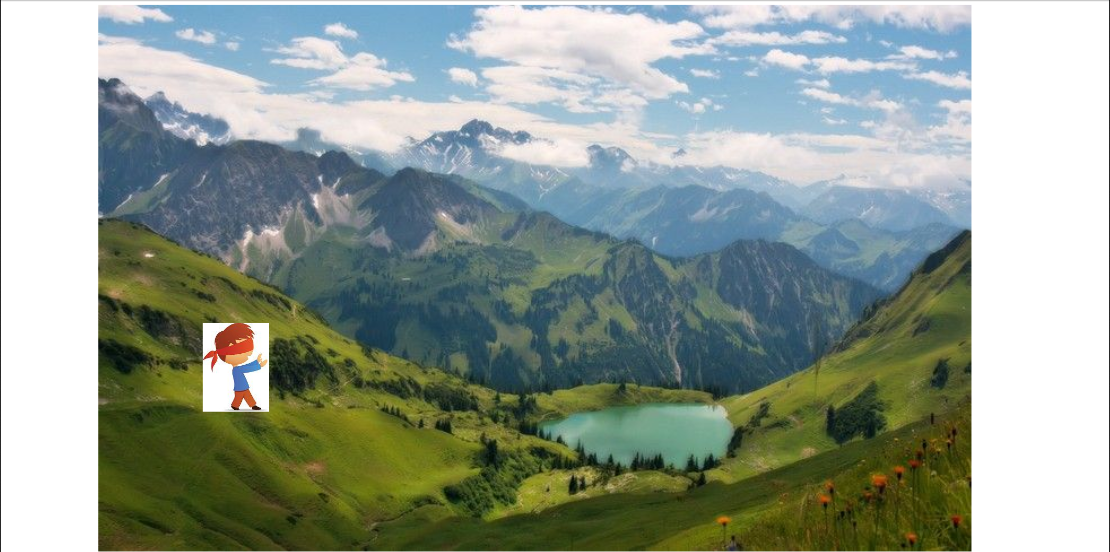
To understand the intuition behind gradient descent, imagine a hiker trying to descend from the top of a mountain to a valley. The hiker‘s objective is to reach the lowest point in the valley, but the terrain is foggy, and the hiker can only assess the steepness of the slope at their immediate position. A reasonable strategy for the hiker would be to look around their current position, determine the direction of the steepest descent, take a step in that direction, and repeat the process until they reach the valley floor.

Mathematically, gradient descent follows a similar principle. Given a cost function J(θ) parameterized by a model‘s parameters θ, the goal is to minimize the cost function by iteratively updating the parameters in the direction of the negative gradient of the cost function with respect to the parameters. The size of the update is controlled by a hyperparameter called the learning rate (α).

The update rule for a parameter θ_i at iteration t is given by:

θ_i(t+1) = θ_i(t) – α * ∂J(θ) / ∂θ_i

where ∂J(θ) / ∂θ_i is the partial derivative of the cost function J(θ) with respect to the parameter θ_i.

How Gradient Descent Works

To gain a deeper understanding of how gradient descent works, let‘s consider a simple example of linear regression. In linear regression, the goal is to find the best-fit line that minimizes the sum of squared errors between the predicted values and the actual values.

Suppose we have a dataset with features X and corresponding target values y. We define our linear regression model as:

ŷ = θ_0 + θ_1 * x

where ŷ is the predicted value, θ_0 is the y-intercept, θ_1 is the slope, and x is the input feature.

The cost function for linear regression is the mean squared error (MSE):

J(θ) = (1/2m) * Σ(ŷ_i – y_i)^2

where m is the number of training examples, ŷ_i is the predicted value for the i-th example, and y_i is the actual value for the i-th example.

To find the optimal values of θ_0 and θ_1 using gradient descent, we initialize them with some random values and iteratively update them using the following equations:

θ_0 := θ_0 – α (1/m) Σ(ŷ_i – y_i)
θ_1 := θ_1 – α (1/m) Σ((ŷ_i – y_i) * x_i)

By repeatedly applying these update rules, the parameters θ_0 and θ_1 gradually converge to their optimal values, minimizing the cost function.

Visualizing Gradient Descent

To visualize the gradient descent process, we can plot the cost function J(θ) as a function of the parameters θ. For simplicity, let‘s consider a cost function with only one parameter θ.

In this plot, the x-axis represents the parameter θ, and the y-axis represents the cost function J(θ). The red curve shows the cost function, and the green dots represent the steps taken by gradient descent.

At each step, gradient descent computes the gradient (slope) of the cost function at the current parameter value and takes a step in the negative direction of the gradient. The size of the step is determined by the learning rate α. This process continues until the algorithm reaches a minimum, where the gradient is close to zero.

Challenges and Considerations in Gradient Descent

While gradient descent is a powerful optimization algorithm, it comes with its own set of challenges and considerations:

1. Non-convex optimization: Gradient descent is guaranteed to converge to the global minimum for convex optimization problems. However, in machine learning, many optimization problems are non-convex, meaning they have multiple local minima. In such cases, gradient descent may get stuck in a suboptimal local minimum.

2. Vanishing or exploding gradients: In deep neural networks, the gradients can become extremely small (vanishing) or extremely large (exploding) during backpropagation. This can cause the optimization process to either slow down significantly or diverge.

3. Choice of learning rate: The learning rate α is a critical hyperparameter in gradient descent. If the learning rate is too small, the algorithm will converge slowly. If the learning rate is too large, the algorithm may overshoot the minimum and diverge.

4. Initialization of parameters: The initial values of the parameters can influence the convergence of gradient descent. Poor initialization can lead to slower convergence or even divergence.

5. Stochastic nature of mini-batch gradient descent: When using mini-batch gradient descent, the gradients are estimated based on a subset of the training data. This introduces noise into the optimization process, which can cause the algorithm to oscillate or converge to a suboptimal solution.

Variants of Gradient Descent

To address the challenges and improve the efficiency of gradient descent, several variants have been proposed. Let‘s explore some of the most popular ones:

1. Stochastic Gradient Descent (SGD): Instead of using the entire training dataset to compute the gradients, SGD uses a single randomly selected example at each iteration. This makes the algorithm faster and allows it to escape local minima more easily. However, SGD can be noisy and may not converge to the exact minimum.

2. Mini-Batch Gradient Descent: Mini-batch gradient descent strikes a balance between batch gradient descent and SGD. It divides the training dataset into small batches and computes the gradients based on each batch. This reduces the noise in the gradients compared to SGD while still being computationally efficient.

3. Gradient Descent with Momentum: Momentum is a technique that helps accelerate gradient descent by adding a fraction of the previous update to the current update. This helps the algorithm gain momentum in the relevant direction and overcome small local minima.

4. Nesterov Accelerated Gradient (NAG): NAG is an extension of gradient descent with momentum. It calculates the gradients not at the current position but at a position slightly ahead in the direction of the momentum. This anticipatory update helps the algorithm converge faster.

5. Adagrad: Adagrad adapts the learning rate for each parameter based on the historical gradients observed for that parameter. It performs larger updates for infrequent parameters and smaller updates for frequent parameters. This is particularly useful when dealing with sparse data.

6. Adadelta: Adadelta is an extension of Adagrad that addresses its monotonically decreasing learning rate. It accumulates the squared gradients over a window and updates the parameters based on the root mean squared (RMS) of the gradients.

7. RMSprop: RMSprop is similar to Adadelta but uses a moving average of the squared gradients instead of a window. It divides the learning rate by the RMS of the recent gradients, allowing the algorithm to adapt to the changing magnitudes of gradients.

8. Adam: Adam (Adaptive Moment Estimation) combines the ideas of momentum and RMSprop. It maintains both a moving average of the gradients (first moment) and a moving average of the squared gradients (second moment). Adam adapts the learning rate for each parameter based on these moments.

Selecting and Tuning Gradient Descent Variants

With so many variants of gradient descent available, it can be overwhelming to choose the right one for your problem. Here are some general guidelines:

• If your dataset is large and redundant, use SGD or mini-batch gradient descent for faster convergence.
• If you have a non-convex optimization problem, momentum-based methods like gradient descent with momentum or NAG can help escape local minima.
• If your data is sparse or your features have varying frequencies, consider using adaptive methods like Adagrad, Adadelta, RMSprop, or Adam.
• When in doubt, start with the Adam optimizer, as it often performs well across a wide range of problems.

Once you have selected a variant, it‘s essential to tune the hyperparameters, such as the learning rate, batch size, and momentum coefficient. You can use techniques like grid search, random search, or Bayesian optimization to find the optimal hyperparameter values.

Gradient Descent in Python

To demonstrate the implementation of gradient descent in Python, let‘s revisit the linear regression example. We‘ll use NumPy for numerical operations and Matplotlib for visualization.

import numpy as np
import matplotlib.pyplot as plt

# Generate random dataset
np.random.seed(42)
X = np.random.rand(100, 1)
y = 2 + 3 * X + np.random.randn(100, 1)

# Initialize parameters
theta = np.random.randn(2, 1)

# Set hyperparameters
learning_rate = 0.1
num_iterations = 1000

# Perform gradient descent
for iteration in range(num_iterations):
    # Compute predicted values
    y_pred = theta[0] + theta[1] * X

    # Compute gradients
    d_theta_0 = 1/m * np.sum(y_pred - y)
    d_theta_1 = 1/m * np.sum((y_pred - y) * X)

    # Update parameters
    theta[0] -= learning_rate * d_theta_0
    theta[1] -= learning_rate * d_theta_1

# Plot results
plt.scatter(X, y)
plt.plot(X, theta[0] + theta[1] * X, color=‘red‘)
plt.xlabel(‘X‘)
plt.ylabel(‘y‘)
plt.title(‘Linear Regression with Gradient Descent‘)
plt.show()

In this example, we generate a random dataset, initialize the parameters randomly, and set the learning rate and number of iterations. We then perform gradient descent by iteratively computing the predicted values, calculating the gradients, and updating the parameters. Finally, we plot the dataset and the best-fit line obtained through gradient descent.

Gradient Descent in Machine Learning

Gradient descent is a fundamental optimization algorithm used in various machine learning algorithms:

1. Linear Regression: As demonstrated in the previous example, gradient descent is used to find the optimal parameters (coefficients) of the linear regression model.

2. Logistic Regression: Gradient descent is employed to minimize the logistic loss function and find the optimal parameters for binary classification problems.

3. Neural Networks: Gradient descent, often in the form of backpropagation, is used to train neural networks by minimizing the loss function with respect to the network‘s weights.

4. Support Vector Machines (SVM): Gradient descent can be used to optimize the objective function of SVMs and find the optimal hyperplane for classification or regression tasks.

5. Recommender Systems: Gradient descent is applied to minimize the error between the predicted ratings and the actual ratings in collaborative filtering-based recommender systems.

These are just a few examples of how gradient descent is utilized in machine learning. Its versatility and effectiveness make it a go-to optimization algorithm for a wide range of machine learning problems.

Conclusion

Gradient descent is a powerful optimization algorithm that forms the backbone of many machine learning algorithms. By iteratively updating the model‘s parameters in the direction of steepest descent, gradient descent enables us to minimize the cost function and find the optimal solution.

In this article, we explored the intuition behind gradient descent, delved into its mathematical formulation, discussed the challenges and considerations, and introduced various variants that address specific issues. We also provided a Python implementation of gradient descent for linear regression and highlighted its applications in different machine learning algorithms.

Armed with this knowledge, you are now well-equipped to apply gradient descent effectively in your own machine learning projects. Remember to experiment with different variants, tune the hyperparameters, and monitor the optimization process to ensure convergence and achieve the best results.

References and Further Reading

1. Ruder, S. (2016). An overview of gradient descent optimization algorithms. arXiv preprint arXiv:1609.04747.
2. Goodfellow, I., Bengio, Y., & Courville, A. (2016). Deep learning. MIT press.
3. Bottou, L., Curtis, F. E., & Nocedal, J. (2018). Optimization methods for large-scale machine learning. Siam Review, 60(2), 223-311.
4. Goh, G. (2017). Why momentum really works. Distill, 2(4), e6.
5. Zeiler, M. D. (2012). ADADELTA: an adaptive learning rate method. arXiv preprint arXiv:1212.5701.