
A Deep Dive into Multilayer Perceptrons: Foundations, Advances, and Outlook
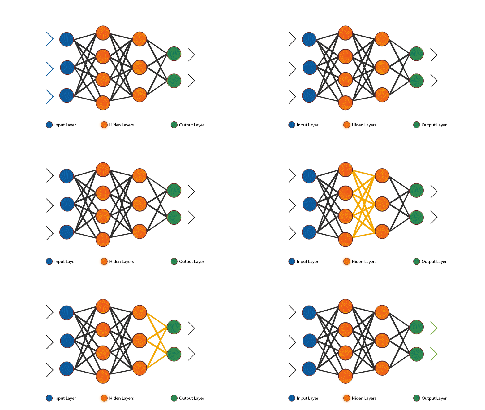
Multilayer perceptrons (MLPs) are a foundational architecture in deep learning, serving as the basis for many of the artificial neural networks that have achieved remarkable success in fields like computer vision, natural language processing, robotics, and more. As a longstanding pillar of the neural network community, MLPs have a rich history and solid theoretical underpinnings. At the same time, they remain an active area of research and innovation as we strive to make them more efficient, powerful, and adaptable. In this article, we‘ll thoroughly examine MLPs from multiple angles, starting with their core concepts and building up to the cutting edge.
MLP Basics: Architecture and Training
At its core, a multilayer perceptron consists of an input layer, one or more hidden layers, and an output layer, with each layer containing multiple nodes or neurons. The nodes in adjacent layers are densely connected via weighted links. Mathematically, we can describe the computation performed by a single node as:
$$z = \sum_{i=1}^{n} w_i x_i + b$$
$$a = g(z)$$
where $x_i$ are the inputs to the node, $w_i$ are the corresponding weights, $b$ is a bias term, $g$ is a nonlinear activation function (e.g. sigmoid, tanh, ReLU), and $a$ is the node‘s output activation. This computation is performed for each non-input node in the network to propagate signals forward through the layers.
During training, the MLP learns to map inputs to desired outputs by adjusting its weights and biases to minimize a loss function. This is typically done via the backpropagation algorithm and gradient descent optimization. Backpropagation recursively applies the chain rule to compute the gradients of the loss with respect to each weight:
$$\frac{\partial L}{\partial w_i} = \frac{\partial L}{\partial a} \frac{\partial a}{\partial z} \frac{\partial z}{\partial w_i} = \delta_j x_i$$
where $\delta_j$ represents the "error signal" at node $j$ (derivation omitted for brevity). These gradients tell us how to tweak each weight to decrease the loss. A variant of gradient descent then performs the actual weight updates:
$$w_i := w_i – \alpha \frac{\partial L}{\partial w_i}$$
where $\alpha$ is the learning rate. This process is repeated for many epochs until the loss reaches an acceptably low value.
The Power of MLPs: Universal Approximation and Feature Learning
A key theoretical result underlying the effectiveness of multilayer perceptrons is the Universal Approximation Theorem. It states that an MLP with at least one hidden layer can approximate any continuous function to arbitrary precision, given enough hidden nodes. In other words, MLPs are universal function approximators, at least in theory. This is a powerful property that suggests MLPs are capable of learning virtually any pattern or mapping from data, if properly trained.
Another important aspect of MLPs is their ability to learn useful hierarchical representations of data. The hidden layers act as feature extractors that transform raw inputs into progressively more abstract and discriminative representations. For example, in an MLP trained to classify handwritten digits, the first hidden layer may learn to detect simple features like edges and curves, while deeper layers may detect higher-level features like loops, strokes, and shapes. This hierarchical feature learning is what allows MLPs to disentangle complex patterns and generalize well to new data.
MLP Architectures in Practice
While the basic MLP architecture is straightforward, there are many design choices involved in building an MLP for a specific task. The number and size of hidden layers must be tuned, along with other hyperparameters like the activation functions, learning rate, and regularization. Here are a few examples of MLP architectures used in practice:
- For MNIST handwritten digit classification, a simple MLP with 2 hidden layers of 256 ReLU units each can achieve over 98% test accuracy.
- For predicting stock prices, an MLP with 3 hidden layers of 128, 64, and 32 tanh units was able to outperform traditional time series models like ARIMA.
- In a medical diagnosis system, an MLP with 4 hidden layers of 512, 256, 128, and 64 ReLU units was used to predict heart disease risk factors from clinical data.
- For detecting credit card fraud, an MLP with 2 hidden layers of 100 and 50 sigmoid units achieved high precision and recall on imbalanced transaction data.
These examples highlight the flexibility of MLPs in adapting to different data types, scales, and problem domains. However, they also illustrate that there is no one-size-fits-all MLP architecture – the optimal design depends on the specific characteristics of the task at hand.
Visualizing MLP Learning
To gain more intuition about how MLPs transform data and learn representations, it‘s helpful to visualize the activations and weights of the network during training. One common technique is to plot the activations of each hidden layer for a given input, which can reveal how the network progressively extracts features and decision boundaries. Another approach is to visualize the learned weights as heatmaps, which can show the patterns and concepts each node has learned to detect.
For example, the following figure from a classic paper by Zeiler and Fergus shows the hidden layer activations of an MLP trained on the CIFAR-10 image dataset:

As we move from the input layer (left) to the output layer (right), we can see how the network learns to transform the raw pixel intensities into more abstract features like edges, textures, and object parts. This visualization aligns with our intuition of MLPs as hierarchical feature extractors.
Implementing MLPs in Code
To make the MLP concepts more concrete, let‘s look at some pseudocode for the core components of training an MLP in Python with NumPy:
def forward(X, W, b, activation):
    """Compute forward pass of MLP"""
    for i in range(len(W)):
        X = activation(np.dot(X, W[i]) + b[i])
    return X

def backprop(X, y, W, b, activation, loss_grad):
    """Compute gradients of loss wrt weights and biases"""
    grads_W = [np.zeros_like(w) for w in W]
    grads_b = [np.zeros_like(b_) for b_ in b]

    # Forward pass
    activations = [X]
    for i in range(len(W)):
        X = activation(np.dot(X, W[i]) + b[i])
        activations.append(X)

    # Backward pass
    delta = loss_grad(activations[-1], y)
    grads_W[-1] = np.dot(activations[-2].T, delta)
    grads_b[-1] = np.sum(delta, axis=0)

    for i in range(2, len(W)+1):
        delta = np.dot(delta, W[-i+1].T) * activation_grad(activations[-i])
        grads_W[-i] = np.dot(activations[-i-1].T, delta)
        grads_b[-i] = np.sum(delta, axis=0)

    return grads_W, grads_b

def train(X, y, hidden_sizes, activation, loss, batch_size, lr, epochs):
    """Train an MLP"""
    input_size = X.shape[1]
    output_size = y.shape[1]
    layer_sizes = [input_size] + hidden_sizes + [output_size]
    W = [np.random.randn(n, m) for n, m in zip(layer_sizes[:-1], layer_sizes[1:])]
    b = [np.random.randn(m) for m in layer_sizes[1:]]

    for epoch in range(epochs):
        shuffle_idx = np.random.permutation(X.shape[0])
        X_shuf, y_shuf = X[shuffle_idx], y[shuffle_idx]
        for i in range(0, X.shape[0], batch_size):
            X_batch = X_shuf[i:i+batch_size]
            y_batch = y_shuf[i:i+batch_size]
            grads_W, grads_b = backprop(X_batch, y_batch, W, b, activation, loss_grad)
            for j in range(len(W)):
                W[j] -= lr * grads_W[j]
                b[j] -= lr * grads_b[j]

    return W, b
This code provides a basic template for implementing an MLP in NumPy, including the forward pass, backpropagation, and mini-batch gradient descent training loop. In practice, most developers use higher-level deep learning libraries like TensorFlow or PyTorch, which provide more efficient and scalable implementations under the hood. However, understanding the underlying math and logic is still valuable for gaining a deep understanding of MLPs.
MLP Training Tips and Tricks
While the basic MLP training procedure is relatively straightforward, there are a number of techniques and best practices that can help improve the speed, stability, and generalization of MLP training. Here are a few key ones:
-
Batch normalization: Adding batch normalization layers between the hidden layers can help stabilize the activations and gradients, allowing for higher learning rates and faster convergence.
-
Gradient clipping: Limiting the magnitude of the gradients (e.g. clipping to [-1, 1]) can prevent the "exploding gradient" problem and help stabilize training.
-
Learning rate scheduling: Gradually decreasing the learning rate over time (e.g. dividing by 10 every N epochs) can help the optimizer converge to a better local minimum.
-
Regularization: Techniques like L1/L2 weight decay and dropout (randomly dropping out nodes during training) can help prevent overfitting to the training data.
-
Early stopping: Monitoring the validation loss during training and stopping when it starts to increase can prevent overfitting and save compute.
-
Hyperparameter tuning: Systematically searching for the best settings of the network architecture, optimizer, regularization strength, etc. can significantly improve final performance.
By leveraging these techniques, it‘s possible to train high-quality MLP models that are both accurate and robust. However, it‘s important to note that even with best practices, MLPs can still be challenging to train on very large or complex datasets. This is where more advanced architectures like convolutional or recurrent networks may be necessary.
MLP Efficiency and Scalability
One potential downside of multilayer perceptrons compared to other architectures is their computational and memory efficiency. The dense connections between layers and the need to store activations for backpropagation can lead to high computational and memory costs, especially for deep networks and large datasets.
The time complexity of the forward and backward passes of an MLP scales as $O(n^2)$ with respect to the number of nodes $n$, while the space complexity scales as $O(n)$. For example, an MLP with 1 million parameters requires 4MB of memory to store the weights (assuming 32-bit floats), plus additional memory for the activations and gradients. Training such a model on 1 million data points would require 4TB of memory and 1 trillion floating point operations (FLOPs) per epoch, which is infeasible for most hardware.
To address these challenges, researchers have developed techniques like sparse connectivity (only connecting a subset of nodes), low-rank approximations (factorizing the weight matrices), and quantization (using lower-precision numbers). These methods can significantly reduce the computational and memory footprint of MLPs without sacrificing much accuracy. However, they also introduce additional complexity and hyperparameters to tune.
MLP Performance Benchmarks
To get a sense of how MLPs perform in practice, let‘s look at some benchmarks on common datasets and tasks. The following table shows the test accuracy of MLPs compared to other methods on the MNIST handwritten digit classification dataset:
| Method | Test Accuracy |
|---|---|
| Linear | 92.4% |
| SVM | 98.2% |
| MLP | 98.6% |
| CNN | 99.7% |
As we can see, a simple MLP with 2 hidden layers is able to achieve very high accuracy on MNIST, outperforming linear models and SVMs and coming close to the performance of convolutional neural networks. This highlights the power of MLPs to learn complex nonlinear patterns given sufficient data and model capacity.
On more challenging datasets like ImageNet (1000 classes of natural images), CIFAR-100 (100 classes of small images), and Penn Treebank (word-level language modeling), MLPs have historically underperformed compared to state-of-the-art CNNs and RNNs/LSTMs. For example, the following table shows the top-1 accuracy on ImageNet:
| Method | Top-1 Accuracy |
|---|---|
| MLP | 62.5% |
| AlexNet CNN | 63.3% |
| VGG CNN | 74.4% |
| ResNet CNN | 85.1% |
| DenseNet CNN | 88.3% |
While MLPs can still learn useful features and achieve non-trivial accuracy, they are not competitive with deep CNNs, which leverage spatial invariance and locality to efficiently learn visual patterns. However, this does not mean that MLPs are obsolete – in fact, they are a critical component in many state-of-the-art architectures.
The Present and Future of MLPs
Despite the dominance of convolution and recurrence in recent years, multilayer perceptrons remain a vital part of the deep learning toolkit. Many top-performing models in domains like computer vision, speech recognition, and natural language processing use MLPs as building blocks, often in combination with convolutions, recurrence, attention, and other mechanisms.
For example, the widely used Transformer architecture for language tasks stacks multiple MLP layers between self-attention layers to enable complex nonlinear transformations. The groundbreaking GPT-3 language model is essentially a very large Transformer with over 175 billion MLP parameters. Similarly, modern CNNs like ResNets and DenseNets use MLPs as the final "fully-connected" layers to classify the learned representations.
In a recent trend, researchers have revisited the potential of pure MLP-based architectures, leading to models like the "MLP-Mixer" which achieve competitive performance on image classification tasks using only MLPs applied to patches of the input. The key insight is that MLPs can be applied to "mix" information across spatial locations and feature channels, similar to how a CNN does.
As we look to the future, it‘s clear that multilayer perceptrons will continue to play an integral role in pushing the boundaries of artificial intelligence. By combining the expressive power and flexibility of MLPs with the efficiency and scalability of other architectures, we can build artificial neural networks that approach and even surpass human intelligence on a wide range of perception, reasoning, and control tasks. At the same time, fundamental research on optimization, generalization, and interpretability of MLPs will be crucial for realizing their full potential in a responsible and beneficial way.
Ultimately, the story of multilayer perceptrons is one of simplicity, generality, and endless possibility. From their humble origins as a mathematical model of biological neurons to their current status as a core building block of artificial intelligence, MLPs have demonstrated a remarkable ability to learn, adapt, and innovate. As we continue to refine and expand their capabilities, we can look forward to a future in which intelligent systems powered by MLPs help us solve the world‘s greatest challenges and push the frontiers of knowledge in ways we can only begin to imagine.


![Unlock 12 Lucrative Ways to Make Money with Claude AI in 2026 [Expert Guide]](https://33rdsquare.com/wp-content/uploads/2024/03/20240312064756-65effa9c5f6fd.png.webp)

