Load a color image

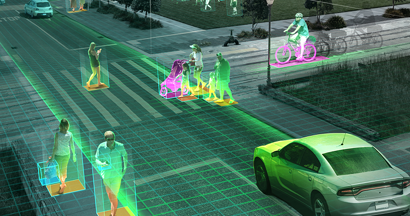
Computer vision has become one of the hottest fields in tech, powering everything from facial recognition and autonomous vehicles to augmented reality and visual search. And if you want to get started with computer vision using Python, there‘s no better place to begin than the Open Source Computer Vision Library – OpenCV.

OpenCV is a massive open-source library for computer vision, machine learning, and image processing that‘s been around since 2000. It contains over 2500 optimized algorithms and is used by tech giants like Google, Microsoft, Intel, IBM, Sony, and Honda. Best of all, it‘s totally free for academic and commercial use!

While OpenCV is available for multiple programming languages, Python has emerged as the go-to language for computer vision and deep learning applications. The combination of Python and OpenCV makes it quick and easy to build powerful computer vision apps.

However, getting started with OpenCV can be daunting, given the sheer number of functions it contains. Understanding which methods to use for which tasks is key to using the library effectively.

In this article, we‘ll walk through 20 of the most important OpenCV functions with Python code examples. By the end, you‘ll be ready to start working on your own computer vision projects!

1. Reading, Writing, and Displaying Images

Before you can manipulate and analyze images, you need to be able to load them into OpenCV. The cv2.imread() function allows you to read images in a variety of formats like JPG, PNG, and TIFF. You simply pass it the path to the image file.

By default, images are loaded in BGR color format. You can specify other options like loading in grayscale or with transparency. Here‘s an example:

import cv2

img = cv2.imread(‘image.jpg‘) 

gray = cv2.imread(‘image.jpg‘, cv2.IMREAD_GRAYSCALE)  

rgba = cv2.imread(‘image.png‘, cv2.IMREAD_UNCHANGED)

To display an image, you use the cv2.imshow() function, specifying the window name and image to display. You can have multiple windows open at once. Use cv2.waitKey() to pause execution until a key is pressed, otherwise the image window will close immediately. cv2.destroyAllWindows() will close any open windows.

cv2.imshow(‘Original‘, img)
cv2.imshow(‘Grayscale‘, gray)
cv2.waitKey(0)
cv2.destroyAllWindows()

Finally, to save a processed image back to disk, use cv2.imwrite():

cv2.imwrite(‘gray_image.jpg‘, gray)

2. Resizing Images

When working with multiple images, it‘s often necessary to make them the same size, typically the input size required by a deep learning model. This can be done with cv2.resize():

resized = cv2.resize(img, (224, 224))

The first argument is the image to resize, and the second is the target dimensions as a tuple of (width, height). By default, OpenCV uses bilinear interpolation, but you can specify other methods like nearest neighbor or bicubic.

3. Image Rotation and Translation

To rotate an image by an arbitrary angle, use cv2.getRotationMatrix2D() to generate a rotation matrix, then apply it with cv2.warpAffine():

(h, w) = img.shape[:2]
center = (w / 2, h / 2)
angle = 45
scale = 1.0
M = cv2.getRotationMatrix2D(center, angle, scale)
rotated = cv2.warpAffine(img, M, (w, h))

This rotates the image by 45 degrees counterclockwise around its center. The scale argument allows you to scale the image up or down at the same time.

Translation shifts an image left/right and up/down. To translate an image by a certain number of pixels, create a translation matrix and apply it with cv2.warpAffine():

M = np.float32([[1, 0, 25], [0, 1, 50]])
translated = cv2.warpAffine(img, M, (img.shape[1], img.shape[0]))  

This shifts the image 25 pixels to the right and 50 pixels down. Rotation and translation are often used for data augmentation to generate additional training examples.

4. Converting Color Spaces

OpenCV supports over 150 color space conversions. The most common are BGR↔RGB, BGR↔Grayscale, and BGR↔HSV. To convert between color spaces, use cv2.cvtColor() and specify the desired conversion code:

gray = cv2.cvtColor(img, cv2.COLOR_BGR2GRAY)
hsv = cv2.cvtColor(img, cv2.COLOR_BGR2HSV) 
rgb = cv2.cvtColor(img, cv2.COLOR_BGR2RGB)

HSV (hue, saturation, value) is often used for color-based segmentation, as it separates the color information (hue) from the intensity (value). This makes it more robust to lighting changes than RGB.

5. Image Thresholding

Thresholding is a segmentation technique that creates a binary image from a grayscale one, with pixel values of 0 or 255. This is useful for separating an object from the background.

Simple thresholding compares each pixel to a fixed threshold value. If the pixel value is greater than the threshold, it‘s set to white (255), otherwise it‘s black (0).

ret, thresh = cv2.threshold(gray, 125, 255, cv2.THRESH_BINARY)

The first argument is the grayscale image, second is the threshold value, third is the maximum value, and fourth is the thresholding type. Other types include THRESH_BINARY_INV, THRESH_TRUNC, THRESH_TOZERO, and THRESH_TOZERO_INV.

For images with varying lighting conditions, adaptive thresholding calculates different thresholds for different image regions. This tends to give better results. You specify the threshold calculation method (mean or Gaussian-weighted) and block size:

adaptive_thresh = cv2.adaptiveThreshold(gray, 255, cv2.ADAPTIVE_THRESH_GAUSSIAN_C, cv2.THRESH_BINARY, 11, 2)

6. Edge Detection

Edge detection is one of the most fundamental operations in computer vision. Edges are points where the image brightness changes sharply. They‘re useful because they often correspond to boundaries of objects.

The most popular edge detection algorithms are Sobel, Laplacian, and Canny. OpenCV provides functions for all of these. Here‘s an example using Canny edge detection:

edges = cv2.Canny(gray, 100, 200)

The arguments are the grayscale image, the lower threshold, and the upper threshold for edge detection. Canny first applies Gaussian smoothing to reduce noise, then finds edges using the Sobel kernel in both horizontal and vertical directions.

7. Image Blurring and Filtering

Blurring, also known as smoothing, is used to reduce noise and detail in an image. It‘s often applied before other operations like edge detection or thresholding. The most common blurring technique is Gaussian blur, which convolves the image with a Gaussian kernel:

blurred = cv2.GaussianBlur(img, (5, 5), 0)

The arguments are the image, the kernel size as a tuple (height, width), and the standard deviation in the X and Y directions. A larger kernel size will blur the image more. Other blurring options in OpenCV include average blurring, median blurring, and bilateral filtering.

Bilateral filtering has the unique property of removing noise while preserving edges, something a Gaussian blur can‘t do. It accomplishes this by using two Gaussian filters: one in the spatial domain, and one in the intensity domain.

8. Contour Detection

Contours are curves joining all the continuous points along a boundary. They‘re useful for shape analysis and object detection/recognition. To find contours, first apply thresholding or edge detection to get a binary image. Then use cv2.findContours():

contours, hierarchy = cv2.findContours(thresh, cv2.RETR_EXTERNAL, cv2.CHAIN_APPROX_SIMPLE)

This finds all the external contours in a binary image using simple approximation, which compresses horizontal, vertical, and diagonal segments into their end points only. To draw the contours on the original image, use cv2.drawContours():

  
cv2.drawContours(img, contours, -1, (0, 255, 0), 2)

This draws all the contours (-1) in green with a thickness of 2 px. You can also specify individual contours to draw by their index.

9. Feature Detection and Matching

Feature detection and matching are used to align different images of the same scene or object, a key step in image stitching, object tracking, and 3D reconstruction. The goal is to find distinctive key points that are invariant to translation, rotation, and scale.

Popular feature detection algorithms include SIFT (Scale-Invariant Feature Transform), SURF (Speeded Up Robust Features), and ORB (Oriented FAST and Rotated BRIEF). While SIFT and SURF are patented, ORB is a good open-source alternative that‘s much faster.

Here‘s an example of detecting and drawing ORB key points:

orb = cv2.ORB_create()
keypoints, descriptors = orb.detectAndCompute(gray, None)
out = img.copy()

out = cv2.drawKeypoints(out, keypoints, None, color=(0, 255, 0))

This creates an ORB object, detects key points in the grayscale image, then draws them on the original as green circles.

To match key points between two images, you first extract their descriptors, then use a matcher like brute-force or FLANN (Fast Library for Approximate Nearest Neighbors):

matcher = cv2.BFMatcher(cv2.NORM_HAMMING, crossCheck=True)
matches = matcher.match(descriptors_1, descriptors_2)
matches = sorted(matches, key = lambda x:x.distance)
out = cv2.drawMatches(img_1, keypoints_1, img_2, keypoints_2, matches[:20], None, flags=2)  

This matches the descriptors of the top 20 ORB key points between two images using brute-force matching with cross-checking. The matches are drawn on a new image for visualization.

10. Face and Object Detection

OpenCV provides pre-trained Haar cascade classifiers for detecting faces, eyes, smiles, and more. It also supports object detection using HOG (Histogram of Oriented Gradients) and SVM (Support Vector Machine).

For face detection, first load the appropriate XML classifier file, then use the detectMultiScale method:

face_cascade = cv2.CascadeClassifier(‘haarcascade_frontalface_default.xml‘)
faces = face_cascade.detectMultiScale(gray, scaleFactor=1.1, minNeighbors=5)
for (x, y, w, h) in faces:
cv2.rectangle(img, (x, y), (x+w, y+h), (0, 255, 0), 2)

This loads the default face detection cascade, detects faces in the grayscale image (returns a list of rectangles), and draws green rectangles around them in the original image. You can tweak the parameters for better accuracy:

• scaleFactor: How much the image size is reduced at each scale
• minNeighbors: How many neighbors each candidate rectangle should have to be considered a face
• minSize: Minimum possible face size, to ignore small detections

Similar code can be used for eye and smile detection by loading the appropriate cascade files. For general object detection, you‘ll need to train your own HOG detector on positive and negative image samples.

11. Deep Learning with OpenCV

In recent years, OpenCV has added support for deep learning networks like Caffe, TensorFlow, and Torch/PyTorch. This allows you to easily load pre-trained models for image classification, object detection, semantic segmentation, and more.

For example, to load a Caffe model for image classification:

net = cv2.dnn.readNetFromCaffe(‘deploy.prototxt‘, ‘model.caffemodel‘)

Then to classify an image:

blob = cv2.dnn.blobFromImage(img, 1, (224, 224), (104, 117, 123))
net.setInput(blob)
predictions = net.forward()
class_id = np.argmax(predictions)

This resizes the input image to 224×224, subtracts the mean BGR values, sets the blob as input to the network, and forward propagates to get the class predictions. The class with the highest score is the winner.

Similar code can be used for object detection models like MobileNet-SSD or YOLO, which return bounding box coordinates in addition to class labels. With semantic segmentation models like UNet, you get a label for every pixel.

The ability to leverage deep learning has made OpenCV an even more powerful tool, lowering the barrier to entry for computer vision applications.

Other Useful Libraries

While OpenCV provides a comprehensive set of computer vision algorithms, there are a few other libraries you should know about:

• NumPy: the fundamental package for numerical computing in Python. OpenCV represents images as multi-dimensional NumPy arrays. Many OpenCV functions expect NumPy arrays as inputs.

• Matplotlib: a plotting library that lets you visualize images, histograms, and other 2D/3D data. Useful for debugging intermediate steps in your computer vision pipeline.

• SciPy: a library for scientific computing, including optimization, linear algebra, integration, and statistics. Some SciPy functions can be used for image processing.

• Scikit-image: an image processing library built on top of NumPy and SciPy. It includes algorithms for segmentation, geometric transformations, color space manipulation, analysis, filtering, feature detection, and more. A good complement to OpenCV.

Learn More

This article has covered some of the most widely used OpenCV functions, but there are many more to explore. The official OpenCV documentation is a great resource, with detailed explanations and code samples in C++ and Python.

To go deeper, check out the free online book "OpenCV-Python Tutorials" and the O‘Reilly book "Learning OpenCV 3 with Python". Adrian Rosebrock‘s website PyImageSearch also has excellent OpenCV tutorials for beginners and experts alike.

The best way to learn computer vision with OpenCV is through hands-on practice. Try implementing the code in this article, then move on to solving real-world problems that interest you. With a little creativity and effort, you‘ll be building powerful computer vision applications in no time!