How to Treat Overfitting in Convolutional Neural Networks

Introduction

Convolutional neural networks (CNNs) have revolutionized the field of computer vision, achieving remarkable performance on tasks like image classification, object detection, and semantic segmentation. However, one common pitfall when training CNNs is overfitting – when a model learns to fit the training data too closely and fails to generalize well to new, unseen examples.

Overfitting occurs when a CNN has learned the noise and peculiarities in the training data to the extent that it negatively impacts the model‘s ability to generalize. The model essentially memorizes the training examples rather than learning the underlying patterns and concepts. Overfitting is more likely with complex models that have a large number of learnable parameters relative to the size of the training data.

There are several tell-tale signs that your CNN is overfitting:

• The model achieves very high accuracy on the training set but much lower accuracy on a held-out validation or test set
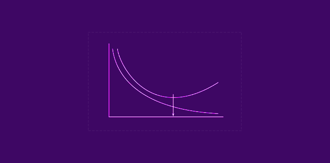
• The training loss continues to decrease with more epochs but the validation loss stagnates or starts increasing
• The gap between training and validation accuracy is significant (e.g. 95% vs 75%)

Fortunately, there are many techniques we can use to combat overfitting and improve a CNN‘s generalization ability. Let‘s dive into some of the most effective approaches.

Data-Centric Approaches

Before jumping into architectural changes or regularization, it‘s important to first look at your data. Having a sufficiently large and diverse training dataset is critical for learning models that generalize well. Here are a few data-centric best practices:

Proper Train/Validation/Test Split

Start by splitting your data into separate training, validation, and test sets. The validation set is used to tune hyperparameters and provide an unbiased estimate of model performance during training. The test set is held out until the very end for final model evaluation. A typical split is 70% training, 15% validation, and 15% test, although the optimal ratio may vary depending on the size of your dataset. Scikit-learn‘s train_test_split function makes this easy:

from sklearn.model_selection import train_test_split
train_imgs, val_imgs, train_labels, val_labels = train_test_split(
imgs, labels, test_size=0.3, random_state=42
)
val_imgs, test_imgs, val_labels, test_labels = train_test_split(
val_imgs, val_labels, test_size=0.5, random_state=42
) 

Data Augmentation

Data augmentation is a technique for artificially increasing the size and diversity of your training set by applying random (but realistic) transformations to the images. This helps expose the model to a wider variety of examples and makes it more robust to variations encountered in the real world. Popular augmentations for images include:

• Random cropping and resizing
• Horizontal/vertical flips
• Rotations
• Color jittering (random changes to brightness, contrast, saturation)
• Adding noise
• Elastic distortions

Many deep learning frameworks have built-in support for data augmentation. For example, in Keras you can use the ImageDataGenerator class:

from tensorflow.keras.preprocessing.image import ImageDataGenerator
datagen = ImageDataGenerator(
rotation_range=20,
zoom_range=0.1,
width_shift_range=0.1,
height_shift_range=0.1,
horizontal_flip=True,
brightness_range=(0.8, 1.2)
)
datagen.fit(train_imgs)

Regularization Methods

Regularization techniques constrain the complexity of a model by adding a penalty term to the loss function during training. This discourages the model from learning overly-complex representations. Two popular regularization methods for neural networks are L1/L2 regularization and dropout.

L1/L2 Regularization

L1 and L2 regularization add a penalty term to the loss function that is proportional to the absolute values (L1) or squared values (L2) of the model‘s weights. L2 regularization is more common and often referred to as "weight decay" in the context of neural networks.

In Keras, you can add L2 regularization to a layer by setting the kernel_regularizer argument:

from tensorflow.keras.regularizers import l2
model.add(Conv2D(32, (3, 3), activation=‘relu‘, kernel_regularizer=l2(0.01)))

L2 regularization pushes the weights towards zero, which can help alleviate overfitting. The hyperparameter (0.01 in this example) controls the strength of the regularization – larger values enforce stronger weight decay.

Dropout

Dropout is a regularization technique that probabilistically "drops out" (i.e. sets to zero) a fraction of the neurons during training. This forces the network to learn redundant representations and prevents over-reliance on any single feature. At test time, all neurons are used but their outputs are scaled down by the dropout probability.

Adding dropout in Keras is straightforward:

from tensorflow.keras.layers import Dropout
model.add(Conv2D(32, (3, 3), activation=‘relu‘))
model.add(Dropout(0.5))

Here a dropout rate of 0.5 is used, meaning each neuron has a 50% chance of being dropped out during training. Typical values range from 0.2 to 0.5.

Early Stopping

Early stopping is a simple but effective regularization technique that stops model training once performance on a validation set starts to degrade. This helps prevent the model from overfitting to the training data.

Keras supports early stopping via a callback:

from tensorflow.keras.callbacks import EarlyStopping
early_stop = EarlyStopping(
monitor=‘val_loss‘, patience=5, restore_best_weights=True
)
history = model.fit(
train_imgs, 
train_labels,
epochs=50, 
validation_data=(val_imgs, val_labels),
callbacks=[early_stop]
)

Here the model will stop training if the validation loss (val_loss) does not improve for 5 consecutive epochs (patience=5). The restore_best_weights parameter ensures the model weights are restored to the values from the epoch with the best validation loss.

Architecture Changes

The architecture of your CNN – the number and size of layers, types of layers used, etc. – plays a big role in its generalization ability. In general, deeper and more complex networks are more prone to overfitting. Two ways to address this are reducing model complexity and improving weight initialization.

Reducing Model Size/Complexity

If your model is severely overfitting, try reducing the depth (number of layers) and width (number of filters/neurons per layer) of your network. You can also use depthwise separable convolutions or 1×1 "bottleneck" layers to reduce the number of parameters.

Global average pooling is another way to decrease model size. Instead of flattening feature maps and passing them to fully-connected layers, you average each feature map to a single value. This greatly reduces the number of parameters:

from tensorflow.keras.layers import GlobalAveragePooling2D
model.add(GlobalAveragePooling2D())
model.add(Dense(num_classes, activation=‘softmax‘))  

Improved Weight Initialization

The initial values of a model‘s weights can impact its ability to learn and generalize. Keras offers several common initializers including Glorot uniform (aka Xavier uniform), Glorot normal, He uniform, and He normal. He initialization often works well for ReLU activation functions:

from tensorflow.keras.layers import Dense
from tensorflow.keras.initializers import he_normal
model.add(Dense(64, activation=‘relu‘, kernel_initializer=he_normal()))

Transfer Learning

Transfer learning is the process of using a model trained on one task as a starting point for a model on a different (but related) task. In the context of CNNs, this typically means using the convolutional layers of a model pre-trained on a large dataset like ImageNet. There are two main approaches:

1. Use the pre-trained CNN as a fixed feature extractor. Pass your images through the pre-trained model and use its output features as input to a new classifier you train from scratch.

2. Fine-tune the pre-trained model. Unfreeze some/all of the layers in the pre-trained model and continue training it on your dataset, typically with a very low learning rate.

The first approach is simpler and less prone to overfitting, while the second allows you to adapt the pre-trained features to your specific dataset. Keras makes transfer learning easy with its pre-trained models:

from tensorflow.keras.applications import VGG16
base_model = VGG16(weights=‘imagenet‘, include_top=False, input_shape=(224, 224, 3))
x = base_model.output
x = GlobalAveragePooling2D()(x)
x = Dense(512, activation=‘relu‘)(x) 
x = Dropout(0.5)(x)
outputs = Dense(num_classes, activation=‘softmax‘)(x)
model = Model(inputs=base_model.input, outputs=outputs)

Here we‘re using VGG16 pre-trained on ImageNet as a feature extractor. We remove the top fully-connected layers (include_top=False), add global average pooling and a couple dense layers on top, and train this new "head" classifier while keeping the VGG16 weights frozen.

Ensembling

Ensembles combine predictions from multiple models to produce a final prediction. This typically results in better generalization than any single model. A simple ensembling method is to train multiple models with different architectures or hyperparameters and average their predictions at test time.

You can also use bagging, where multiple models are trained on different random subsets of the training data. At test time, you average the models‘ predictions. This reduces variance and overfitting because each model sees a different "view" of the data.

Monitoring Performance

Keeping a close eye on your model‘s performance during training is critical for identifying and addressing overfitting. The key metrics to watch are:

• Training vs validation loss: Plot both training and validation loss after each epoch. If validation loss starts increasing while training loss is still decreasing, your model is likely overfitting.

• Training vs validation accuracy: Similarly, plot training and validation accuracy over time. A substantial gap between the two indicates overfitting.

Keras‘ fit method returns a history object that contains this data:

history = model.fit(...)
loss = history.history[‘loss‘]
val_loss = history.history[‘val_loss‘] 

It‘s also helpful to visualize the learned features at different layers in your network, either by plotting the filter weights or activations in response to an input image. This gives insight into whether your model is learning meaningful features or just memorizing patterns.

Conclusion

Overfitting is a common challenge when training CNNs, but there are many tools at your disposal to mitigate it. The most important pieces of the puzzle are:

1. Use a large, diverse training dataset and apply data augmentation
2. Add regularization to your model in the form of L1/L2 regularization, dropout, or early stopping
3. Reduce model complexity or use transfer learning if your model is severely overfitting
4. Combine predictions from multiple models in an ensemble
5. Closely monitor training and validation metrics to catch overfitting early

The key is to experiment with different combinations of these approaches and see what works best for your specific problem. Don‘t be afraid to iterate and try new things – finding the right balance between model complexity and generalization is as much an art as it is a science. Above all, always keep your end goal in mind and prioritize techniques that demonstrably improve performance on unseen data. Happy training!