Predicting Using Linear Regression in R: A Complete Guide (2026)

Linear regression is one of the most fundamental and widely used tools in data science and machine learning. It allows you to model and predict relationships between variables. Whether you want to forecast sales, analyze factors influencing employee retention, or estimate housing prices, linear regression is a powerful technique to have in your analytics toolkit.
In this comprehensive guide, we‘ll dive deep into how linear regression works and walk through detailed examples of building linear models to make predictions in R. By the end, you‘ll be equipped with the knowledge and skills to apply linear regression to a variety of real-world problems.
Let‘s get started!
What is Linear Regression?
At its core, linear regression is a statistical method that models the relationship between a dependent variable (also called the response or outcome) and one or more independent variables (also called features or predictors). It finds the line of best fit through your data points to capture the general trend.
More specifically, linear regression estimates the coefficients in a linear equation:
y = β0 + β1×1 + β2×2 + … + βnxn
where:
- y is the dependent variable
- x1, x2, …, xn are the independent variables
- β0 is the y-intercept (value of y when all x = 0)
- β1, β2, …, βn are the coefficients that describe the effect each x has on y
The goal is to find the coefficients that minimize the differences between the observed y values and the y values predicted by the equation. This is accomplished mathematically using the least squares method.
There are two main types of linear regression:
- Simple linear regression – one independent variable
- Multiple linear regression – two or more independent variables
Assumptions of Linear Regression
For the estimates from linear regression to be valid and reliable, several key assumptions must be met:
- Linearity – there is a linear relationship between X and Y
- Independence – observations are independent of each other (no autocorrelation)
- Normality – residuals are normally distributed
- Equal variances – residuals have constant variance at every level of X (homoscedasticity)
It‘s important to check these assumptions using diagnostic plots of the residuals after fitting a linear model. If the assumptions are severely violated, the model may be biased or misleading.
Building Linear Regression Models in R
R makes it very easy to build and diagnose linear regression models. The general steps are:
- Import and explore the data
- Visualize relationships between variables
- Fit the model with lm()
- Check model assumptions
- Interpret model coefficients
- Use model to make predictions
Let‘s see this process in action with an example. We‘ll use a dataset on air pollution and mortality in U.S. cities.
Simple Linear Regression
First, we‘ll import the data into R:
data(usair)
head(usairpollution)
Next, let‘s visualize the relationship between the two variables we‘re interested in – mean annual pollution (SO2) and mean annual mortality rate:
plot(usairpollution$SO2, usairpollution$Mort)There appears to be a positive linear relationship, so a simple linear regression model is appropriate.
Now we‘ll fit the model using the lm() function:
model <- lm(Mort ~ SO2, data = usairpollution)
summary(model)
The output shows that SO2 is a significant predictor of mortality rate (p < 0.001). For every unit increase in SO2, the mortality rate increases by 0.2646 on average. The model explains about 12% of the variance in mortality rate (R2 = 0.1245).
We can check the residual plots to assess if the model assumptions hold:
par(mfrow = c(2,2))
plot(model)
The plots indicate that the assumptions of linearity, normality, and equal variances are reasonably met. There are no major concerns.
Finally, let‘s use the model to predict mortality rates for specific SO2 levels:
newdata = data.frame(SO2 = c(10,50,100))
predict(model, newdata)
The model predicts mortality rates of 952, 966, and 979 per 100,000 for SO2 levels of 10, 50, and 100 respectively.
Multiple Linear Regression
Now let‘s see how to build a multiple linear regression model. We‘ll add two more predictors – mean annual rainfall and mean January temperature.
First fit the model:
model2 = lm(Mort ~ SO2 + Rain + JanTemp, data=usairpollution)
summary(model2)
The output indicates that adding these predictors improves the fit – the model now explains about 34% of the variance in mortality rate (R2 = 0.3412). However, JanTemp is not a significant predictor (p = 0.77).
With multiple predictors, it‘s important to check for multicollinearity – high correlations among predictors that can cause problems. We can use the variance inflation factor (VIF):
library(car)
vif(model2)
VIF values greater than 5 or 10 indicate serious multicollinearity. In this case, there are no major issues.
We can use stepwise selection to systematically add or remove predictors and find the best model:
step(model2, direction="both")The procedure settles on a model with just SO2 and Rain as the most parsimonious and effective.
Lastly, let‘s check the model assumptions again:
par(mfrow = c(2,2))
plot(model2)
No red flags in the diagnostic plots. The model is good to go!
Advantages of Linear Regression
- Simple to understand and explain to others
- Fast to compute, even with millions of data points
- Coefficients directly describe how each predictor affects the outcome
- Highly interpretable – easy to extract insights about relationships between variables
- Provides a measure of uncertainty around estimates
Disadvantages of Linear Regression
- Assumes linear relationships between X and Y – may oversimplify complex patterns
- Sensitive to outliers which can drastically change the fit
- Prone to overfit with a large number of predictors
- Can‘t automatically capture interactions between predictors
- Doesn‘t perform well with highly correlated predictors (multicollinearity)
Applications of Linear Regression
Linear regression has a multitude of applications across business, healthcare, science, economics and more. Some common use cases include:
- Predicting sales based on advertising spend, promotions, etc.
- Analyzing factors that affect employee performance or retention
- Modeling real estate prices based on house features
- Estimating patient medical costs from diagnostic and treatment variables
- Quantifying relationships between chemical properties and biological activity of potential drugs
- Forecasting economic trends from leading indicators
The versatility and simplicity of linear regression make it an indispensable tool for deriving insights from data.
Tips for Applying Linear Regression
- Plot the data first to visually check for linearity
- Code categorical predictors as dummy variables
- Remove or correct outliers and high leverage points
- Check model assumptions and use weighted least squares if needed
- Be cautious in extrapolating predictions beyond the range of the original data
- Don‘t infer causation from correlation – associations alone don‘t prove cause and effect
The Future of Linear Regression
Linear regression remains a foundational technique, but it continues to evolve. Some recent developments include:
- Regularized regression (Ridge, Lasso) to handle high-dimensional data and multicollinearity
- Generalized linear models to model non-normal outcomes
- Robust regression methods that are less sensitive to outliers
- Bayesian linear regression that incorporates prior information
- Linear mixed models to analyze nested or repeated measures data
As data grows in size and complexity, we can expect linear regression to adapt to meet new challenges.
In conclusion, linear regression is a core competency for anyone working with data. With its simplicity, interpretability, and extensibility, it has stood the test of time. By mastering the fundamentals of linear regression in R, you can solve a wide range of real-world problems and uncover valuable insights. Keep building on this knowledge, and happy modeling!