Progressive Growing GAN (ProGAN): A Deep Dive into High-Resolution Image Synthesis

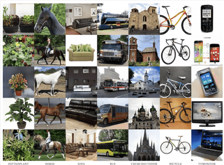
Generative Adversarial Networks (GANs) have revolutionized the field of computer vision, enabling the creation of highly realistic synthetic images. However, traditional GANs often struggle with training instability and generating high-resolution images. Progressive Growing GAN (ProGAN), introduced by Karras et al. in 2017, addresses these challenges by introducing a novel training methodology that progressively grows the generator and discriminator models, allowing for the stable synthesis of high-resolution images.

Understanding GANs

Before diving into ProGAN, let‘s briefly review the basics of GANs. A GAN consists of two neural networks: a generator and a discriminator. The generator takes random noise as input and attempts to generate realistic images, while the discriminator tries to distinguish between real images from the training dataset and fake images produced by the generator. The two networks are trained simultaneously in a minimax game, where the generator aims to fool the discriminator, and the discriminator aims to correctly classify real and fake images.

Challenges in Training GANs

Despite their success, traditional GANs face several challenges:

1. Training instability: GANs are notoriously difficult to train, often suffering from issues like mode collapse, where the generator produces a limited variety of images, and vanishing gradients, where the feedback from the discriminator becomes uninformative.

2. Difficulty in generating high-resolution images: As the resolution of generated images increases, the training becomes more unstable, and the quality of the generated images often degrades.

ProGAN aims to address these challenges by introducing a progressive growing scheme and several architectural innovations.

Key Innovations in ProGAN

1. Progressive growing: ProGAN starts by generating low-resolution images (e.g., 4×4) and gradually increases the resolution by adding new layers to the generator and discriminator. This allows the models to learn coarse-level features first and then progressively refine the details as the resolution increases.

2. Minibatch standard deviation: To improve the discriminator‘s ability to detect generated images, ProGAN introduces a minibatch standard deviation layer that computes the standard deviation of activations across the batch dimension and adds it as a new feature map to the discriminator.

3. Pixel-wise normalization: To stabilize the training, ProGAN applies pixel-wise normalization to the generator‘s activations, which normalizes each pixel‘s feature vector to unit length. This helps prevent the escalation of feature magnitudes during training.

4. Equalized learning rate: ProGAN uses a modified weight initialization and scaling technique called equalized learning rate, which ensures that the dynamic range of the weights remains the same throughout the training process, further improving stability.

Training ProGAN

The training process of ProGAN can be summarized as follows:

1. Start with a low resolution (e.g., 4×4) and train the generator and discriminator until convergence.
2. Fade in new layers to double the resolution (e.g., 8×8) and continue training.
3. Repeat step 2 until the desired resolution is reached (e.g., 1024×1024).

During the transition to a higher resolution, ProGAN uses a weighted sum of the previous resolution‘s output and the new resolution‘s output, gradually shifting the weight towards the new resolution over several iterations. This smooth transition helps maintain stability during the resolution increase.

Implementing ProGAN in PyTorch

To implement ProGAN in PyTorch, you‘ll need to define custom layers like WSConv2d (weight-scaled convolution) and PixelNorm, as well as the generator and discriminator architectures that incorporate these layers. Here‘s a simplified example of the generator:

class Generator(nn.Module):
    def __init__(self, z_dim, in_channels, img_channels):
        super(Generator, self).__init__()
        self.initial = nn.Sequential(
            PixelNorm(),
            nn.ConvTranspose2d(z_dim, in_channels, 4, 1, 0),
            nn.LeakyReLU(0.2),
            WSConv2d(in_channels, in_channels, kernel_size=3, stride=1, padding=1),
            nn.LeakyReLU(0.2),
            PixelNorm(),
        )
        self.initial_rgb = WSConv2d(in_channels, img_channels, kernel_size=1, stride=1, padding=0)
        self.prog_blocks, self.rgb_layers = nn.ModuleList([]), nn.ModuleList([self.initial_rgb])

        for i in range(len(factors) - 1):
            conv_in_c = int(in_channels * factors[i])
            conv_out_c = int(in_channels * factors[i + 1])
            self.prog_blocks.append(ConvBlock(conv_in_c, conv_out_c))
            self.rgb_layers.append(WSConv2d(conv_out_c, img_channels, kernel_size=1, stride=1, padding=0))

    def fade_in(self, alpha, upscaled, generated):
        return torch.tanh(alpha * generated + (1 - alpha) * upscaled)

    def forward(self, x, alpha, steps):
        out = self.initial(x)
        if steps == 0:
            return self.initial_rgb(out)
        for step in range(steps):
            upscaled = F.interpolate(out, scale_factor=2, mode="nearest")
            out = self.prog_blocks[step](upscaled)
        final_upscaled = self.rgb_layers[steps - 1](upscaled)
        final_out = self.rgb_layers[steps](out)
        return self.fade_in(alpha, final_upscaled, final_out)

The discriminator follows a similar structure but in reverse, downsampling the input image and using minibatch standard deviation.

Training Tips and Best Practices

1. Use appropriate hyperparameters: Experiment with different learning rates, batch sizes, and regularization techniques to find the optimal configuration for your task.

2. Monitor training progress: Use tools like TensorBoard to visualize the training progress, including losses, generated images, and model graphs.

3. Employ the truncation trick: During inference, you can control the trade-off between sample quality and diversity by truncating the input latent vector. This can help generate higher-quality samples at the cost of reduced variety.

Applications and Future Directions

ProGAN has been successfully applied to various tasks, such as generating high-resolution face images, creating synthetic datasets for data augmentation, and performing style transfer. However, there are still limitations and areas for future research:

1. Further improving training stability and scalability to enable the generation of even higher-resolution images.
2. Incorporating additional constraints or loss functions to improve the semantic consistency and controllability of the generated images.
3. Extending the progressive growing approach to other types of data, such as audio and video, to enable high-quality generation in those domains.

Conclusion

Progressive Growing GAN (ProGAN) has made significant strides in stabilizing the training of GANs and enabling the generation of high-resolution images. By progressively growing the generator and discriminator, employing architectural innovations like minibatch standard deviation and pixel-wise normalization, and using techniques like equalized learning rate, ProGAN has set a new standard for image synthesis with GANs.

As research in this field continues to advance, we can expect further improvements in the quality, diversity, and controllability of generated images, as well as the extension of these techniques to other domains. With its powerful capabilities and potential applications, ProGAN remains an essential tool in the arsenal of computer vision and deep learning practitioners.