A Comprehensive Guide to Topic Modeling with Latent Semantic Analysis using Python

Introduction

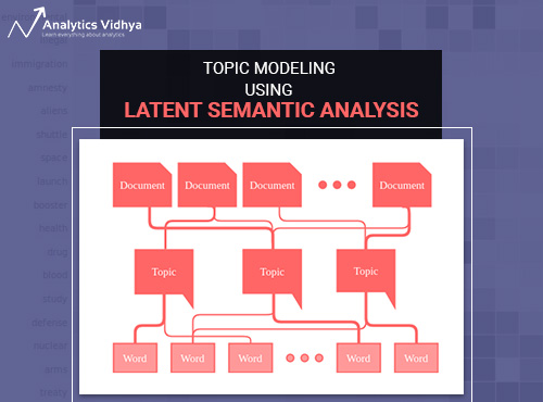
Topic modeling is an incredibly useful technique in natural language processing (NLP) for discovering hidden semantic structures in a body of text. It allows us to automatically cluster documents into groups and extract meaningful themes or "topics" from them based on the frequency and distribution of words. This has a wide range of practical applications, from organizing large document collections to identifying key topics in social media posts, customer reviews, and more.

One of the foundational techniques for topic modeling is latent semantic analysis (LSA), also known as latent semantic indexing (LSI). LSA leverages matrix factorization methods like singular value decomposition (SVD) to uncover the underlying relationships between words and documents. Despite being one of the older topic modeling approaches, LSA remains widely used due to its simplicity, effectiveness, and ease of implementation.

In this guide, we‘ll walk through the step-by-step process of performing topic modeling with LSA using Python. We‘ll cover everything from data preparation to model building to visualization and interpretation of the results. Whether you‘re a complete beginner to NLP or have some experience, this tutorial will equip you with a solid understanding of LSA and practical skills for applying it to your own projects. Let‘s dive in!

Overview of Latent Semantic Analysis

At a high level, LSA works by constructing a matrix representation of a text corpus and using linear algebra techniques to reduce its dimensionality while preserving the most important semantic information. The key steps are:

1. Construct a document-term matrix where each row represents a document and each column represents a unique word (term) in the corpus. The values are typically weighted counts like TF-IDF.

2. Perform truncated singular value decomposition on the matrix to factorize it into three matrices: $U$ (document-topic matrix), $\Sigma$ (diagonal matrix of singular values), and $V^T$ (term-topic matrix).

3. Reduce the dimensionality by only keeping the top $k$ singular values and vectors, effectively mapping documents and terms to a lower-dimensional "topic space".

4. Interpret the resulting matrices, where each row of $U$ represents a document‘s topic distribution and each row of $V^T$ represents a topic‘s word distribution.

Mathematically, the SVD of a matrix $A$ is defined as:

$A = U \Sigma V^T$

where $U$ and $V$ are orthonormal matrices (left and right singular vectors) and $\Sigma$ is a diagonal matrix of singular values. By truncating these matrices to keep only the top $k$ components, we get the rank-$k$ approximation:

$A_k = U_k \Sigma_k V_k^T$

This provides a way to approximate the original matrix while capturing the most important patterns and structure in the data. Intuitively, LSA can be thought of as a way to uncover the "latent" semantic relationships between words and documents based on their co-occurrence patterns.

Implementing LSA in Python

Now that we have a high-level understanding of how LSA works, let‘s walk through the steps to implement it in Python with the help of some common NLP and machine learning libraries.

1. Reading and Inspecting Text Data

The first step is to load our text data into memory so we can work with it. Python provides many convenient ways to read text data, whether it‘s stored in a file, database, or coming from an API. For simplicity, we‘ll use a sample dataset of documents in plain text format.

import os

# Assuming documents are stored in a "data" directory as .txt files 
documents = []
for filename in os.listdir("data"):
    with open(os.path.join("data", filename), "r") as file:
        documents.append(file.read())

print(f"Loaded {len(documents)} documents")
print("Example document:")
print(documents[0][:300] + "...")  

It‘s always a good idea to do some basic exploration of the data to check for any issues and get a sense of what we‘re working with. We can print out the number of documents loaded, inspect a sample document, and even visualize the distribution of document lengths.

2. Data Preprocessing

Raw text data is messy and not directly suitable for analysis. We need to clean and preprocess it to remove irrelevant information and convert it into a standard format. This typically involves:

• Tokenization: splitting the text into individual words or tokens
• Lowercasing: converting all characters to lowercase
• Removing punctuation, numbers, and special characters
• Removing stopwords: filtering out common words like "the", "and", "is"
• Stemming/Lemmatization: reducing words to their base or dictionary form

Python‘s NLTK library provides convenient tools for most of these steps:

import nltk
from nltk.corpus import stopwords
from nltk.stem import WordNetLemmatizer

stop_words = set(stopwords.words(‘english‘))
lemmatizer = WordNetLemmatizer()

def preprocess(text):
    # Tokenize and lowercase
    words = nltk.word_tokenize(text.lower())

    # Remove non-alphanumeric characters
    words = [word for word in words if word.isalpha()]

    # Remove stopwords and lemmatize
    words = [lemmatizer.lemmatize(word) for word in words if word not in stop_words]

    return words

processed_docs = [preprocess(doc) for doc in documents]

3. Creating Document-Term Matrix

The next step is to convert our preprocessed text data into a matrix representation we can perform mathematical operations on. The most common format is a document-term matrix where each row represents a document and each column represents a unique word.

We can use sklearn‘s CountVectorizer to construct this matrix, optionally specifying parameters like the max/min document frequency and number of features to consider:

from sklearn.feature_extraction.text import CountVectorizer

# Fit vectorizer on processed documents
vectorizer = CountVectorizer(max_df=0.7, min_df=2, max_features=5000)  
doc_term_matrix = vectorizer.fit_transform(processed_docs)

print(f"Document-term matrix shape: {doc_term_matrix.shape}")

The values in this matrix are raw counts of how often each word appears in each document. However, raw counts can be biased towards longer documents and don‘t account for the importance of words. A common solution is to use TF-IDF (term frequency-inverse document frequency) weighting instead:

from sklearn.feature_extraction.text import TfidfTransformer

# Transform counts into TF-IDF weights
tfidf_transformer = TfidfTransformer()
tfidf_matrix = tfidf_transformer.fit_transform(doc_term_matrix)

TF-IDF increases the weight of words that are frequent in a document but rare across the corpus, capturing their specificity and importance. This matrix is now ready for topic modeling.

4. Performing Singular Value Decomposition

The heart of LSA is truncated singular value decomposition to factorize the document-term matrix into separate document-topic and term-topic matrices. We can easily do this using sklearn‘s TruncatedSVD:

from sklearn.decomposition import TruncatedSVD

# Create LSA model and fit to TF-IDF matrix
lsa_model = TruncatedSVD(n_components=10)  
lsa_model.fit(tfidf_matrix)

# Get document-topic and term-topic matrices
doc_topic_matrix = lsa_model.transform(tfidf_matrix)  
topic_term_matrix = lsa_model.components_

The key parameter is n_components which specifies the number of topics (and thus dimensions) to retain. This is essentially a hyperparameter that needs to be tuned for each dataset, either manually using domain knowledge or automatically through cross-validation and evaluation metrics like perplexity or coherence.

5. Interpreting Topics

Once we have the low-dimensional topic representation, the final step is to interpret the topics and see if they capture meaningful themes in the data. We can do this by looking at the most important terms associated with each topic in the term-topic matrix:

# Get feature names from vectorizer
feature_names = vectorizer.get_feature_names()

# Print top terms for each topic
for topic_idx, topic in enumerate(topic_term_matrix):
    print(f"Topic {topic_idx}:")
    print(" ".join([feature_names[i] for i in topic.argsort()[:-10 - 1:-1]]))

This prints out the top 10 terms for each topic in descending order of importance. By examining these terms, we can get a sense of what each topic represents and how well the model has captured the underlying themes in the data. Keep in mind that interpreting topics is somewhat subjective and may require domain expertise.

In addition to the top terms, we can also look at the distribution of topics across documents to see how prevalent each topic is and which documents are most associated with each topic. This can be done by examining the document-topic matrix:

import numpy as np

# Get topic distribution for each document
doc_topic_dist = doc_topic_matrix / np.sum(doc_topic_matrix, axis=1, keepdims=True)

# Print top documents for each topic
for topic_idx in range(doc_topic_matrix.shape[1]):
    print(f"Topic {topic_idx}:")
    top_doc_indices = doc_topic_dist[:,topic_idx].argsort()[::-1][:5]
    for doc_index in top_doc_indices:
        print(f"- Document {doc_index}: {documents[doc_index][:50]}...")

This prints out the top 5 documents associated with each topic, giving us a more concrete sense of what the topics represent in the actual text data.

6. Visualizing Topics

Finally, we can visualize the topics to get an intuitive sense of how they relate to each other and how documents cluster around them. One common technique is to use dimensionality reduction methods like PCA or t-SNE to plot the high-dimensional topic vectors in 2D space:

from sklearn.manifold import TSNE
import matplotlib.pyplot as plt

# Reduce dimensionality of document-topic matrix
tsne_model = TSNE(n_components=2, perplexity=30, random_state=42)
tsne_coordinates = tsne_model.fit_transform(doc_topic_dist)

# Plot documents color-coded by dominant topic
dominant_topic = np.argmax(doc_topic_dist, axis=1)
plt.figure(figsize=(10, 8))
plt.scatter(tsne_coordinates[:,0], tsne_coordinates[:,1], c=dominant_topic, cmap=‘viridis‘)
plt.colorbar(ticks=range(doc_topic_matrix.shape[1]), label=‘Dominant Topic‘)
plt.xlabel(‘t-SNE Dimension 1‘), plt.ylabel(‘t-SNE Dimension 2‘)
plt.title(‘Document Clustering by Dominant Topic‘)
plt.show()

This plots each document as a point in 2D space, color-coded by its dominant topic. Documents that are close together should be semantically similar and associated with the same topics. The overall shape of the clusters can reveal interesting patterns in the data.

Pros and Cons of LSA

LSA is a powerful and widely used technique for topic modeling, but it‘s important to be aware of its strengths and limitations. Some of the key advantages of LSA include:

• Computational efficiency and scalability to large datasets
• Ability to handle synonymy and polysemy (different words with similar meanings)
• Unsupervised approach requiring no labeled data or prior knowledge

However, LSA also has some drawbacks and assumptions that may not always hold:

• Assumes a linear relationship between words and documents, which may be overly simplistic
• Requires choosing the optimal number of topics, which can be challenging
• Lacks probabilistic interpretation and may produce negative values
• Sensitive to preprocessing steps and weighting schemes

For certain use cases, more advanced topic modeling techniques like Latent Dirichlet Allocation (LDA) or neural network-based approaches like lda2vec may be preferred. However, LSA remains a solid choice as a baseline method, especially for initial exploration of a text corpus.

Conclusion

In this guide, we‘ve covered the essential concepts and steps for performing topic modeling with latent semantic analysis using Python. We started by discussing the motivation and intuition behind LSA, as well as its mathematical formulation using singular value decomposition. We then walked through a practical example of implementing LSA on a sample text dataset, including data loading, preprocessing, matrix construction, model fitting, and interpretation/visualization of the resulting topics.

To summarize, the key steps in the LSA workflow are:

1. Load and preprocess text data
2. Construct a document-term matrix (e.g. using TF-IDF)
3. Perform truncated SVD to get document-topic and term-topic matrices
4. Interpret topics by examining top terms and document distributions
5. Visualize topic clusters in low-dimensional space

While LSA is not without limitations, it remains a valuable tool in the NLP practitioner‘s toolkit for uncovering hidden thematic structure in text data. Its relative simplicity and efficiency make it a great choice for initial explorations and building baseline models. That said, it‘s important to be aware of its assumptions and drawbacks, and to consider alternative techniques like LDA when needed.

We‘ve only scratched the surface of what‘s possible with topic modeling and LSA in this guide. Some additional directions to explore include:

• Tuning model hyperparameters like number of topics via cross-validation
• Incorporating more advanced preprocessing with lemmatization, phrase detection, etc.
• Comparing and evaluating different topic modeling approaches
• Using learned topic vectors as features for supervised machine learning tasks
• Applying topic modeling to other data types like images, audio, and time series

I hope this guide has given you a solid foundation in LSA and topic modeling, and equipped you with practical skills to apply these techniques to your own projects. Don‘t hesitate to dive deeper into the underlying math, experiment with different implementations, and extend these ideas to new domains. With the right tools and understanding, you‘ll be well on your way to extracting valuable insights from even the largest and most complex text datasets.