Understanding Confidence Intervals with Python: A Complete Guide
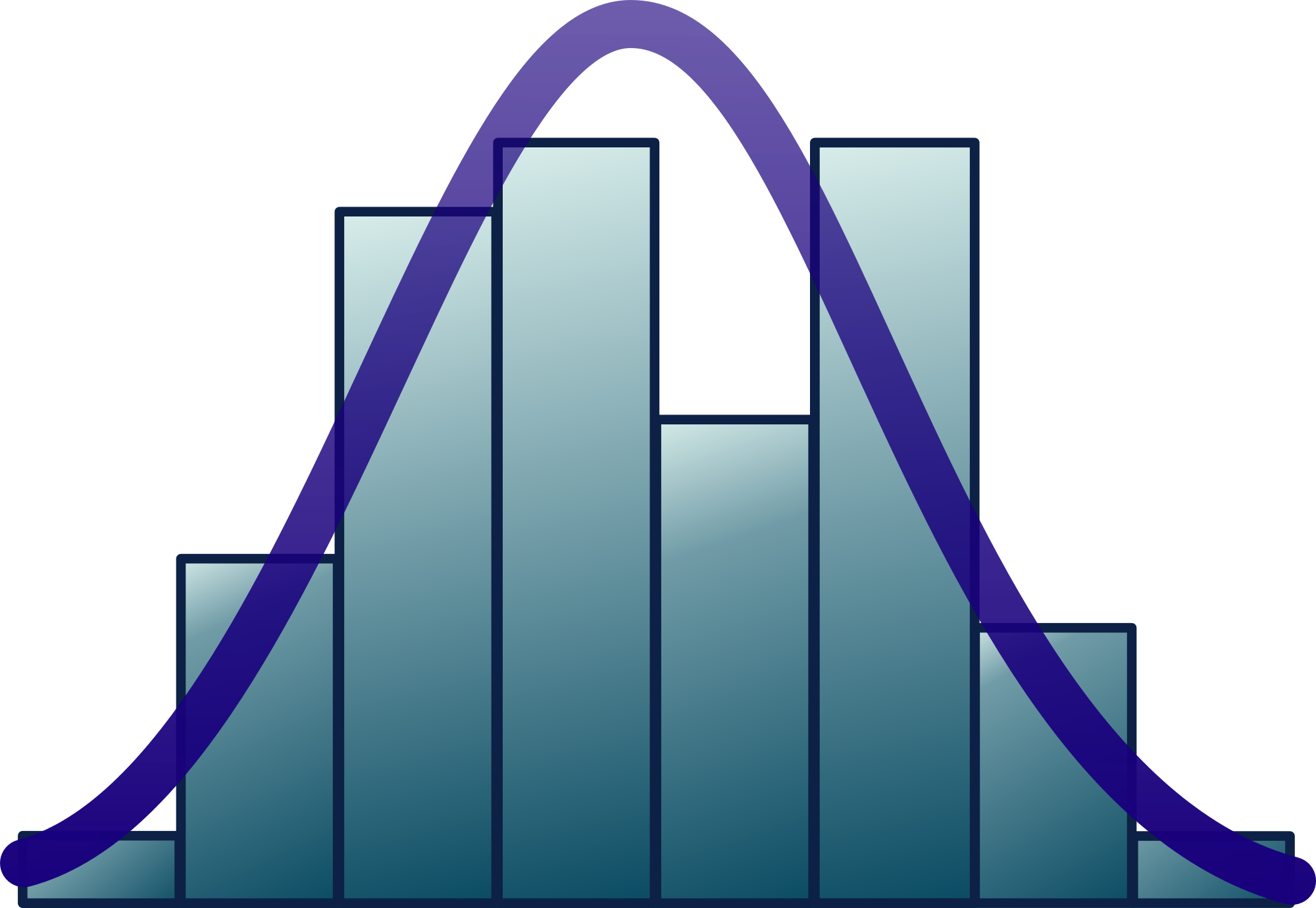
Confidence intervals are a fundamental tool in statistics for quantifying uncertainty in estimates based on sample data. Instead of just providing a single point estimate like a sample mean, a confidence interval gives a range of plausible values for the true population parameter. Confidence intervals help you make more robust conclusions from your data.
In this guide, we‘ll take an in-depth look at confidence intervals and how to calculate them using Python. We‘ll cover the intuition behind confidence intervals, the assumptions required, the difference between z-intervals and t-intervals, and how to interpret the results. We‘ll also explore the relationship between confidence intervals and hypothesis testing, potential pitfalls to watch out for, and real-world applications.
By the end of this article, you‘ll have a solid understanding of what confidence intervals are, when to use them, how to compute them with Python, and how to communicate your findings effectively. Let‘s dive in!
What is a Confidence Interval?
A confidence interval is a range of values that‘s likely to contain a population parameter with a certain level of confidence, based on a sample from that population. It takes the general form:
Estimate ± Margin of Error
Where the estimate is typically a sample statistic like the mean, and the margin of error represents the uncertainty in the estimate. The margin of error depends on factors like the sample size, variability in the data, and desired confidence level.
Common confidence levels are 90%, 95%, and 99%. For instance, a 95% confidence interval for a population mean can be interpreted as: "If we took many samples and constructed a 95% confidence interval from each sample, about 95% of those intervals would contain the true population mean."
Importantly, the confidence level represents the reliability of the method, not the probability that a particular interval contains the population parameter. A specific interval either includes the parameter value or it doesn‘t.
Assumptions for Confidence Intervals
To construct a valid confidence interval, the underlying data should satisfy certain assumptions:
-
Independence: The sample should be randomly selected and independent. Each data point shouldn‘t influence the others.
-
Sample size: The sample size should be large enough for the central limit theorem to apply. A common rule of thumb is n > 30.
-
Normality: For smaller samples, the population data should be approximately normally distributed. For large samples, this assumption is less critical due to the central limit theorem.
Keep these assumptions in mind as we walk through the calculations. If they are violated, the interpretation of the confidence interval may not be reliable.
Confidence Interval for a Population Mean
One of the most common applications of confidence intervals is estimating a population mean. The formula depends on whether the population standard deviation is known (z-interval) or unknown (t-interval).
Let‘s first consider the case where the population standard deviation σ is known. The confidence interval is given by:
X̄ ± z* · σ/√n
Where:
- X̄ is the sample mean
- z* is the critical z-score corresponding to the confidence level
- σ is the population standard deviation
- n is the sample size
The critical z-score can be found using a standard normal table or Python‘s stats functions. For example, for a 95% confidence interval, z* = 1.96.
In practice, the population standard deviation is rarely known. In this case, we use the sample standard deviation s as an estimate for σ and calculate a t-interval:
X̄ ± t* · s/√n
Where t* is the critical t-score with n-1 degrees of freedom. The t-distribution is similar to the standard normal distribution but has heavier tails, accounting for the extra variability from using s.
Calculating Confidence Intervals in Python
Let‘s see how to calculate confidence intervals for a population mean in Python. We‘ll use the scipy.stats module for the critical values and math functions.
Suppose we have a sample of 50 students‘ test scores with a mean of 80 and standard deviation of 10. We want to calculate a 99% confidence interval for the population mean.
import math
from scipy.stats import norm, t

n = 50
x_bar = 80
s = 10
confidence = 0.99

# Calculate the critical t-value
degrees_freedom = n - 1
t_crit = t.ppf((1 + confidence) / 2, degrees_freedom)

# Calculate the margin of error
margin_error = t_crit * s / math.sqrt(n)

# Construct the confidence interval
lower = x_bar - margin_error
upper = x_bar + margin_error

print(f"99% confidence interval: ({lower:.2f}, {upper:.2f})")
# Output: 99% confidence interval: (76.41, 83.59)
We first calculate the critical t-value using scipy.stats.t.ppf(). This function takes the desired cumulative probability and degrees of freedom. Since we want a two-sided interval, we use (1 + confidence) / 2.
Next, we calculate the margin of error by multiplying the critical t-value, sample standard deviation, and a factor of 1/√n.
Finally, we construct the lower and upper bounds of the interval by subtracting and adding the margin of error to the sample mean.
The output shows that we are 99% confident the true population mean test score falls between 76.41 and 83.59.
One-Sided Confidence Intervals
So far, we‘ve considered two-sided confidence intervals, which extend symmetrically below and above the sample statistic. In some cases, you may want a one-sided interval that only bounds the parameter in one direction.
For instance, suppose you want to be 95% confident that the true mean is at least some value. In this case, you would use a one-sided lower bound:
X̄ – t* · s/√n
Where t* now corresponds to the 95th percentile of the t-distribution, rather than the 97.5th percentile used for a two-sided interval. In Python, you can calculate this with t.ppf(0.95, n-1).
Similarly, for a one-sided upper bound:
X̄ + t* · s/√n
One-sided intervals can provide more precision if you are only interested in bounding the parameter in one direction. However, they should be used cautiously, as they don‘t provide information about values in the other direction.
Confidence Intervals for a Population Proportion
In addition to means, we often want to estimate population proportions from sample data. For instance, what proportion of voters support a candidate based on a poll? Or what fraction of manufactured items are defective?
The confidence interval formula for a population proportion p is:
p̂ ± z* · √(p̂(1-p̂)/n)
Where:
- p̂ is the sample proportion
- z* is the critical z-score for the desired confidence level
- n is the sample size
For this interval to be valid, the sample size should be large enough so that np̂ > 10 and n(1-p̂) > 10. This ensures the sampling distribution of p̂ is approximately normal.
Here‘s how to calculate a confidence interval for a proportion in Python:
from scipy.stats import norm

n = 500
p_hat = 0.42
confidence = 0.95

# Calculate the critical z-value
z_crit = norm.ppf((1 + confidence) / 2)

# Calculate the margin of error
margin_error = z_crit * math.sqrt(p_hat * (1 - p_hat) / n)

# Construct the confidence interval
lower = p_hat - margin_error
upper = p_hat + margin_error

print(f"95% confidence interval: ({lower:.3f}, {upper:.3f})")
# Output: 95% confidence interval: (0.383, 0.457)
The steps are similar to the mean case, but we use the standard normal distribution for the critical value and a slightly different formula for the standard error.
The output shows that based on a sample of 500 where 42% had the attribute of interest, we are 95% confident that the true population proportion is between 0.383 and 0.457.
Confidence Intervals for Non-Normal Data
The confidence intervals we‘ve covered so far rely on the normality assumption for the underlying population or sampling distribution. But what if your data is skewed or has outliers?
One option is to use a non-parametric method like the bootstrap. Bootstrapping involves repeated resampling from the observed data to construct an empirical distribution of the statistic. Confidence intervals are then derived from the percentiles of this distribution.
Here‘s a quick example of a bootstrap confidence interval for the median:
import numpy as np

def bootstrap_median_ci(data, confidence=0.95, n_boots=1000):
    medians = []
    for i in range(n_boots):
        boot_sample = np.random.choice(data, size=len(data), replace=True)
        medians.append(np.median(boot_sample))

    return np.percentile(medians, [(1 - confidence) / 2 * 100, (1 + confidence) / 2 * 100])

# Generate some skewed data
data = np.random.exponential(scale=1.0, size=100)

lower, upper = bootstrap_median_ci(data)
print(f"95% bootstrap CI for median: ({lower:.2f}, {upper:.2f})")
# Output: 95% bootstrap CI for median: (0.62, 1.14)
The idea is to resample with replacement from the original data many times (n_boots) and calculate the median for each resample. The confidence interval is then estimated from the empirical percentiles of these resampled medians.
Bootstrap intervals don‘t make strong distributional assumptions, making them a flexible alternative when the data is non-normal. However, they can be computationally intensive and may require a large sample size to perform well.
Interpreting Confidence Intervals
Confidence intervals provide a way to quantify the uncertainty in an estimate, but they are often misinterpreted. Here are a few key points to keep in mind:
-
A 95% confidence interval does not mean there is a 95% probability the true parameter lies in the interval. The parameter is fixed, and the interval either contains it or not. The 95% refers to the long-run proportion of intervals that would contain the parameter if the sampling process was repeated.
-
The width of the interval reflects the precision of the estimate. Narrower intervals indicate more precise estimates, while wider intervals suggest greater uncertainty. Factors that affect precision include the sample size, variability in the data, and confidence level.
-
Confidence intervals provide a range of plausible values for the parameter but don‘t prove any particular value is the true value. They should be interpreted as a measure of uncertainty, not a definitive statement.
-
The confidence level (e.g., 95%) represents the long-run reliability of the method, not the probability for a specific interval. It is a common misinterpretation to think a 95% confidence interval has a 95% chance of containing the parameter.
By keeping these points in mind, you can avoid common misinterpretations and communicate your results more accurately.
Confidence Intervals and Hypothesis Testing
Confidence intervals are closely related to hypothesis tests. In fact, you can often use a confidence interval to draw conclusions about a hypothesis test.
For instance, suppose you want to test the null hypothesis that a population mean equals some value μ0. If a 95% confidence interval for the mean does not contain μ0, you can reject the null hypothesis at the 0.05 significance level. Conversely, if the interval includes μ0, you fail to reject the null.
This relationship provides a visual way to interpret hypothesis tests and p-values. If the confidence interval is far from the null value, the p-value will be small, and vice versa.
However, confidence intervals provide additional information beyond a p-value. They show the range of compatible values and the precision of the estimate. This can lead to more nuanced conclusions than simply rejecting or failing to reject a null hypothesis.
Potential Limitations
While confidence intervals are a valuable tool, they have some potential limitations and pitfalls to be aware of:
-
Confidence intervals are based on a sample and may not capture the full population variability, especially for small or biased samples.
-
The interpretation of confidence intervals relies on the sampling method and assumptions. If the data violate assumptions like independence or normality, the intervals may be misleading.
-
Confidence intervals don‘t account for other sources of error like measurement error, data entry mistakes, or sampling bias. They only quantify the uncertainty due to random sampling.
-
Comparing confidence intervals between groups can suggest differences, but it‘s not a formal hypothesis test. Overlapping intervals do not necessarily imply a non-significant difference.
Understanding these limitations can help you use confidence intervals appropriately and avoid over-interpreting the results.
Real-World Applications
Confidence intervals have numerous applications across fields like science, engineering, business, and public policy. Some examples include:
-
A medical study reporting the effect of a drug on blood pressure with a 95% confidence interval, to show the range of likely treatment effects.
-
A quality control engineer using a confidence interval to estimate the proportion of defective products in a manufacturing process.
-
A market researcher constructing a confidence interval for the mean satisfaction rating of a product, to understand consumer preferences.
-
A political pollster reporting a confidence interval for the proportion of voters supporting a candidate, to predict election outcomes.
In each case, the confidence interval provides a way to quantify and communicate the uncertainty in the findings, which is crucial for decision making.
Conclusion
Confidence intervals are a powerful tool for quantifying uncertainty and making inferences about population parameters. By providing a range of plausible values, they give a more complete picture than a single point estimate.
In this guide, we‘ve covered the key concepts behind confidence intervals, including the formulas for means and proportions, the assumptions required, and how to calculate them in Python. We‘ve also discussed how to interpret confidence intervals correctly, their relationship to hypothesis testing, and some potential limitations.
Remember, a confidence interval is a statement about the reliability of the estimation method, not the specific parameter value. By understanding the proper interpretation and assumptions, you can use confidence intervals to draw more robust conclusions from your data.
I encourage you to practice calculating and interpreting confidence intervals on your own datasets. Consider how they can enhance your data analysis and communication of results. With a solid grasp of confidence intervals, you‘ll be well-equipped to quantify uncertainty and make informed decisions based on your data.
Further Reading: