Convolutional Neural Network Pytorch | CNN Using Pytorch

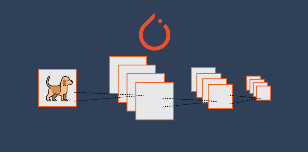
Building Image Classification Models with Convolutional Neural Networks in PyTorch

Introduction
Image classification is a fundamental task in computer vision, with applications ranging from object recognition to medical diagnosis. In recent years, deep learning techniques, particularly convolutional neural networks (CNNs), have revolutionized the field of image classification, achieving state-of-the-art results on various benchmark datasets.

In this blog post, we will explore how to build an image classification model using CNNs in PyTorch, a popular open-source deep learning framework. We will walk through the process step-by-step, from loading and preprocessing the data to defining the model architecture, training the model, and evaluating its performance. By the end of this tutorial, you will have a solid understanding of how to apply CNNs for image classification tasks using PyTorch.

Why Convolutional Neural Networks?
Traditional neural networks, such as multi-layer perceptrons (MLPs), have been used for image classification tasks in the past. However, they have several limitations when it comes to processing image data:

1. Spatial information: MLPs treat each pixel independently and do not consider the spatial relationships between pixels. This means they cannot effectively capture the local patterns and structures present in images.

2. Parameter inefficiency: MLPs require a large number of parameters to process high-dimensional image data, leading to increased computational complexity and a higher risk of overfitting.

Convolutional neural networks address these limitations by incorporating two key concepts: convolutional layers and pooling layers.

Convolutional layers apply a set of learnable filters to the input image, capturing local patterns and features at various scales. These filters are shared across the entire image, allowing the network to learn translation-invariant features. This parameter sharing also reduces the total number of parameters in the model compared to fully-connected layers.

Pooling layers downsample the feature maps produced by convolutional layers, reducing the spatial dimensions while retaining the most important information. This helps to make the model more robust to small translations and distortions in the input image.

By stacking multiple convolutional and pooling layers, CNNs can learn hierarchical representations of the input image, from low-level features like edges and textures to high-level features like object parts and shapes. This hierarchical learning allows CNNs to effectively capture the complex patterns and structures present in image data, making them well-suited for image classification tasks.

PyTorch: A Deep Learning Framework
PyTorch is an open-source deep learning framework developed by Facebook‘s AI Research lab. It provides a flexible and intuitive interface for building and training neural networks using the Python programming language.

Some key features of PyTorch include:

1. Dynamic computation graphs: PyTorch allows you to define computational graphs on-the-fly, enabling dynamic network architectures and easy debugging.

2. GPU acceleration: PyTorch provides seamless GPU support, allowing you to easily train models on NVIDIA GPUs for faster computations.

3. Rich ecosystem: PyTorch has a growing ecosystem of libraries and tools built on top of it, covering various domains such as computer vision, natural language processing, and reinforcement learning.

4. Easy-to-use APIs: PyTorch offers a clean and intuitive API for building and training neural networks, making it accessible to both beginners and experienced practitioners.

In the following sections, we will leverage the power of PyTorch to build and train a CNN for image classification.

Loading and Preprocessing the Data
The first step in any machine learning project is to load and preprocess the data. For this tutorial, we will use the CIFAR-10 dataset, which consists of 60,000 32×32 color images in 10 classes, with 6,000 images per class. The classes include objects such as airplanes, cars, birds, cats, etc.

To load the CIFAR-10 dataset in PyTorch, we can use the torchvision library, which provides easy access to popular datasets and pre-trained models. Here‘s how to load the data:

import torch
import torchvision
import torchvision.transforms as transforms

# Define the transformations to be applied to the data
transform = transforms.Compose(
    [transforms.ToTensor(),
     transforms.Normalize((0.5, 0.5, 0.5), (0.5, 0.5, 0.5))])

# Load the CIFAR-10 training dataset
trainset = torchvision.datasets.CIFAR10(root=‘./data‘, train=True,
                                        download=True, transform=transform)
trainloader = torch.utils.data.DataLoader(trainset, batch_size=64,
                                          shuffle=True, num_workers=2)

# Load the CIFAR-10 testing dataset  
testset = torchvision.datasets.CIFAR10(root=‘./data‘, train=False,
                                       download=True, transform=transform)
testloader = torch.utils.data.DataLoader(testset, batch_size=64,
                                         shuffle=False, num_workers=2)

In this code snippet, we first define the transformations to be applied to the data using the transforms module from torchvision. We convert the images to PyTorch tensors and normalize the pixel values to have zero mean and unit variance. This preprocessing step helps the model converge faster during training.

Next, we load the CIFAR-10 training and testing datasets using the CIFAR10 class from torchvision.datasets. We specify the root directory to store the downloaded data, whether to download the dataset if it‘s not already present, and the transformations to apply. We then create data loaders for both the training and testing datasets, which allow us to efficiently load the data in batches during training and evaluation.

Defining the CNN Architecture
With the data loaded and preprocessed, we can now define the architecture of our CNN model. Here‘s an example of a simple CNN architecture for CIFAR-10 image classification:

import torch.nn as nn
import torch.nn.functional as F

class Net(nn.Module):
    def __init__(self):
        super(Net, self).__init__()
        self.conv1 = nn.Conv2d(3, 32, 3)
        self.pool = nn.MaxPool2d(2, 2)
        self.conv2 = nn.Conv2d(32, 64, 3)
        self.fc1 = nn.Linear(64 * 6 * 6, 256)
        self.fc2 = nn.Linear(256, 84)
        self.fc3 = nn.Linear(84, 10)

    def forward(self, x):
        x = self.pool(F.relu(self.conv1(x)))
        x = self.pool(F.relu(self.conv2(x)))
        x = x.view(-1, 64 * 6 * 6)
        x = F.relu(self.fc1(x))
        x = F.relu(self.fc2(x))
        x = self.fc3(x)
        return x

net = Net()

This CNN architecture consists of two convolutional layers followed by two fully-connected layers. The first convolutional layer has 32 filters of size 3×3, while the second convolutional layer has 64 filters of size 3×3. We apply ReLU activation and max pooling after each convolutional layer to introduce non-linearity and reduce the spatial dimensions.

After the convolutional layers, we flatten the feature maps and pass them through two fully-connected layers with ReLU activation. The final fully-connected layer has 10 output units, corresponding to the 10 classes in the CIFAR-10 dataset.

The forward method defines the forward pass of the model, specifying how the input data flows through the layers to produce the output predictions.

Training the Model
With the model architecture defined, we can now train the model on the CIFAR-10 training dataset. Here‘s how to train the model using PyTorch:

import torch.optim as optim

criterion = nn.CrossEntropyLoss()
optimizer = optim.SGD(net.parameters(), lr=0.001, momentum=0.9)

for epoch in range(10):  # loop over the dataset multiple times

    running_loss = 0.0
    for i, data in enumerate(trainloader, 0):
        # get the inputs; data is a list of [inputs, labels]
        inputs, labels = data

        # zero the parameter gradients
        optimizer.zero_grad()

        # forward + backward + optimize
        outputs = net(inputs)
        loss = criterion(outputs, labels)
        loss.backward()
        optimizer.step()

        # print statistics
        running_loss += loss.item()
        if i % 500 == 499:    # print every 500 mini-batches
            print(‘[%d, %5d] loss: %.3f‘ %
                  (epoch + 1, i + 1, running_loss / 500))
            running_loss = 0.0

print(‘Finished Training‘)

In this code snippet, we first define the loss function (cross-entropy loss) and the optimizer (stochastic gradient descent with momentum). We then loop over the training dataset for a specified number of epochs.

For each mini-batch of data, we perform the following steps:

1. Clear the gradients of all optimized parameters.
2. Forward pass: Compute the output predictions by passing the inputs through the model.
3. Compute the loss between the predicted outputs and the true labels.
4. Backward pass: Compute the gradients of the loss with respect to the model parameters.
5. Update the model parameters using the optimizer.

We also print the running loss every 500 mini-batches to monitor the training progress.

Evaluating the Model
After training the model, we can evaluate its performance on the CIFAR-10 testing dataset to see how well it generalizes to unseen data. Here‘s how to evaluate the model:

correct = 0
total = 0
with torch.no_grad():
    for data in testloader:
        images, labels = data
        outputs = net(images)
        _, predicted = torch.max(outputs.data, 1)
        total += labels.size(0)
        correct += (predicted == labels).sum().item()

print(‘Accuracy of the network on the 10000 test images: %d %%‘ % (
    100 * correct / total))

In this code snippet, we loop over the testing dataset and compute the output predictions for each mini-batch of images. We then compare the predicted labels with the true labels and count the number of correct predictions. Finally, we print the overall accuracy of the model on the testing dataset.

Improving Model Performance
There are several techniques you can use to improve the performance of your CNN model:

1. Data augmentation: Apply random transformations to the training images, such as rotation, flipping, cropping, and scaling, to increase the diversity of the training data and reduce overfitting.

2. Transfer learning: Use a pre-trained CNN model, such as VGG or ResNet, as a feature extractor and fine-tune it on your specific dataset. This allows you to leverage the learned features from a large-scale dataset and adapt them to your task.

3. Hyperparameter tuning: Experiment with different hyperparameters, such as learning rate, batch size, and number of epochs, to find the optimal configuration for your model.

4. Regularization techniques: Apply regularization methods, such as L1/L2 regularization or dropout, to prevent overfitting and improve generalization.

5. Ensemble methods: Train multiple models with different architectures or initializations and combine their predictions using methods like averaging or voting to improve the overall performance.

Conclusion
In this blog post, we explored how to build an image classification model using convolutional neural networks in PyTorch. We covered the key concepts of CNNs, including convolutional layers and pooling layers, and discussed their advantages over traditional neural networks for image data.

We walked through a step-by-step tutorial on loading and preprocessing the CIFAR-10 dataset, defining the CNN architecture, training the model, and evaluating its performance. We also discussed various techniques to improve model performance, such as data augmentation, transfer learning, and hyperparameter tuning.

By following this tutorial, you should now have a solid understanding of how to apply CNNs for image classification tasks using PyTorch. You can further expand upon this knowledge by experimenting with different architectures, datasets, and techniques to build more advanced and accurate models.

Remember, building effective deep learning models is an iterative process that requires experimentation, analysis, and refinement. Keep exploring, keep learning, and don‘t be afraid to try new ideas!

I hope this blog post has been informative and helpful in your journey to mastering convolutional neural networks and image classification with PyTorch. Happy coding!