20 Questions to Test Your Skills on Dimensionality Reduction (PCA)

Introduction

As datasets continue to grow larger and more complex, dimensionality reduction techniques like Principal Component Analysis (PCA) have become essential tools for data scientists and machine learning practitioners. PCA allows us to summarize high-dimensional data using a smaller set of representative variables while retaining most of the original information.

In this article, we‘ll dive deep into the key concepts behind PCA and dimensionality reduction through a set of 20 questions. Whether you‘re brushing up on your skills or preparing for a technical interview, these questions will test your understanding of PCA from the fundamentals to more advanced applications. Let‘s get started!

1. What is dimensionality reduction? Why is it important?

Dimensionality reduction refers to the process of reducing the number of features or variables in a dataset while preserving as much of the relevant information as possible. In machine learning, datasets often contain a large number of dimensions (features), which can lead to several issues:

• Increased computational complexity and longer training times
• Higher risk of overfitting the model to noise in the data
• Difficulty visualizing and interpreting high-dimensional data
• The "curse of dimensionality" where more dimensions require exponentially more data to generalize accurately

Dimensionality reduction techniques aim to alleviate these problems by projecting the data into a lower-dimensional subspace that captures the most important patterns and structures. This leads to simpler models, faster processing, improved generalization, and easier interpretation and visualization of the data.

2. Give an overview of PCA.

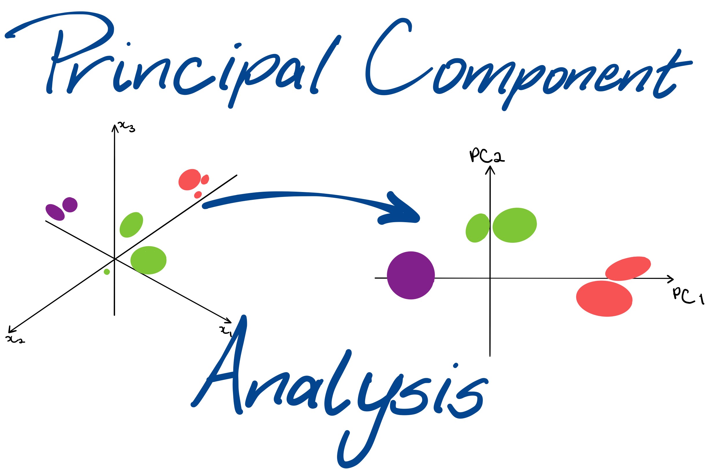
Principal Component Analysis (PCA) is one of the most widely used dimensionality reduction techniques. It is an unsupervised learning method that linearly transforms the data into a new coordinate system where the axes (principal components) are ordered by the amount of variance they explain in the data.

The first principal component captures the direction of maximum variance, the second captures the remaining variance in the orthogonal direction, and so on. By projecting the data onto the top K principal components, we can reduce the dimensionality while preserving the most important information.

PCA has the desirable property of being deterministic – there are no random initializations or risk of getting stuck in local optima. The principal components are uniquely determined by the data.

3. What are the steps in the PCA algorithm?

The PCA algorithm can be broken down into the following steps:

1. Standardize the data (mean=0, variance=1 for each feature)
2. Compute the covariance matrix of the standardized data
3. Find the eigenvectors and eigenvalues of the covariance matrix
4. Sort the eigenvectors by their eigenvalues in decreasing order
5. Choose the top K eigenvectors to form the projection matrix W
6. Transform the original data using X_new = X • W

The transformed data X_new will have K dimensions, where each dimension corresponds to one of the top eigenvectors (principal components). The eigenvectors form the columns of the projection matrix W.

4. Is it necessary to standardize the data before PCA?

Yes, it is generally recommended to standardize the data before applying PCA, especially if the features have different scales or units. Standardization ensures that each feature has zero mean and unit variance.

If the features are not standardized, the high-variance features will dominate the principal components, even if they are not the most informative. This can lead to a suboptimal projection that fails to preserve the important structures in the data.

There are some cases where standardization may not be necessary, such as when all the features are already on the same scale (e.g. image pixel intensities between 0-255). However, standardization is still a good default practice for most applications of PCA.

5. What is the importance of rotating the components in PCA?

The principal components in PCA are orthogonal (perpendicular) to each other by construction. However, in some cases, it can be beneficial to rotate the components while preserving their orthogonality. This is known as rotating the principal components.

Rotation helps to find a more interpretable set of components where each component aligns closely with a subset of the original features. Rotated components are often easier to interpret because they tend to have high loadings on a smaller number of features and near-zero loadings on the rest.

Some popular rotation methods include varimax, quartimax, and equamax rotation. These methods aim to simplify the component structure and aid in interpretation, but they do not change the overall subspace or the amount of variance explained by the components.

If we don‘t rotate the components, the raw principal components may not align well with the original features, making them harder to interpret. However, the choice of rotation ultimately depends on the goals of the analysis and the domain knowledge of the practitioner.

6. What are the key assumptions of PCA?

PCA makes a few important assumptions about the data:

1. Linearity: PCA assumes that the data can be well-approximated by a linear subspace. If the data lies on a nonlinear manifold, PCA may not be able to capture the true structure.

2. High signal-to-noise ratio: PCA assumes that the important patterns in the data have high variance compared to the noise. If the data is very noisy, the principal components may just capture the noise instead of the signal.

3. Multivariate normality: For statistical inference on the principal components (e.g. computing confidence intervals), PCA assumes that the data follows a multivariate normal distribution. However, this assumption is not necessary for just using PCA as a dimensionality reduction tool.

4. Sufficient sample size: To get stable estimates of the covariance matrix and the principal components, PCA requires a sufficient number of samples relative to the number of dimensions. A common rule of thumb is to have at least 5-10 times as many samples as dimensions.

If these assumptions are violated, PCA may not be the most appropriate technique, and other methods like kernel PCA, manifold learning, or autoencoders may be more suitable.

7. What happens when the eigenvalues are roughly equal in PCA?

In PCA, the eigenvalues of the covariance matrix represent the amount of variance explained by each principal component. If all the eigenvalues are roughly equal, it means that all the principal components explain a similar amount of variance in the data.

In this case, PCA may not be very useful for dimensionality reduction, because there is no clear way to select a smaller subset of components that capture most of the information. All the components are equally important, so discarding any of them would lose a significant amount of information.

Equal eigenvalues can occur when the features are uncorrelated and have similar variances. In such cases, PCA just rotates the data to a new orthogonal basis but does not reduce the dimensionality effectively.

If you encounter roughly equal eigenvalues, it may be a sign that PCA is not the right tool for your data. You may need to consider other dimensionality reduction techniques or feature selection methods that can handle uncorrelated or equally important features.

8. What are the properties of principal components?

The principal components in PCA have several important properties:

1. Orthogonality: The principal components are orthogonal (perpendicular) to each other. This means that they represent independent directions of variance in the data.

2. Sorting by variance: The principal components are sorted in decreasing order of their corresponding eigenvalues, which represent the amount of variance explained by each component. The first principal component captures the most variance, followed by the second, and so on.

3. Linear combinations of original features: Each principal component is a linear combination of the original features, where the coefficients (loadings) determine the weight of each feature in the component.

4. Uniqueness: The principal components are uniquely determined by the data, up to a sign flip. If you run PCA multiple times on the same data, you will always get the same components (assuming the same normalization and convention for eigenvalue ordering).

5. Dimensional coverage: The principal components span the same subspace as the original data. If you use all the components (without discarding any), you can perfectly reconstruct the original data from the projected data.

These properties make principal components a powerful tool for data compression, visualization, and feature extraction. By understanding these properties, you can better interpret the results of PCA and use them effectively in your analysis.

Example: PCA on a 2D dataset

To illustrate the steps of PCA, let‘s consider a simple example with a 2D dataset: {(-3,-3), (-1,-1), (1,1), (3,3)}.

Step 1: Standardize the data

Since the data is already centered around the origin (0,0), we don‘t need to subtract the mean. The standard deviation of both dimensions is √20 = 4.472. So we divide each value by 4.472:

X_std = [[-0.671, -0.671],
[-0.224, -0.224],
[ 0.224, 0.224],
[ 0.671, 0.671]]

Step 2: Compute the covariance matrix

The covariance matrix is:

Cov(X_std) = [[ 1.0, 1.0],
[ 1.0, 1.0]]

Step 3: Find the eigenvectors and eigenvalues

The eigenvalues are λ1 = 2.0 and λ2 = 0.0.
The corresponding eigenvectors are:
v1 = [0.707, 0.707] (1st principal component)
v2 = [-0.707, 0.707] (2nd principal component)

Step 4: Project the data onto the top K eigenvectors

If we choose K=1, we project the data onto the first principal component:

X_pca = X_std • v1
= [[-0.949],
[-0.316],
[ 0.316],
[ 0.949]]

The data has been reduced to 1 dimension while preserving the maximum variance.

Advantages of dimensionality reduction

• Mitigates the curse of dimensionality by requiring less data to learn models
• Reduces computational and memory costs for storing and processing the data
• Helps visualize high-dimensional data in 2D or 3D plots
• Extracts the most informative features and discards noise or redundant features
• Improves model performance by reducing overfitting and increasing interpretability

Disadvantages of dimensionality reduction

• May lose important information if too many dimensions are discarded
• Transformed features may be hard to interpret in the original space
• Some methods have high computational complexity for very high-dimensional data
• Unsupervised methods do not consider the target variable, so the reduced features may not be optimal for supervised learning
• Results may be sensitive to the choice of parameters (e.g. number of components)

Latest developments and applications of PCA

As of 2024, PCA continues to be a widely used technique for dimensionality reduction and feature extraction. Some recent developments include:

• Randomized PCA: A faster algorithm for computing the top principal components, especially useful for massive datasets that don‘t fit in memory.
• Robust PCA: An extension that can handle outliers and corrupted data, useful for anomaly detection and image processing.
• Kernel PCA: A nonlinear version of PCA that can capture more complex patterns by mapping the data to a higher-dimensional space.
• Tensor PCA: Generalization of PCA to higher-order tensors, useful for multi-dimensional data like videos and fMRI scans.
• Incremental PCA: Allows updating the principal components efficiently as new data arrives, useful for online learning and streaming data.

PCA is widely used in various domains, including:

• Computer vision: Face recognition, object detection, image compression
• Bioinformatics: Gene expression analysis, population genetics, drug discovery
• Neuroscience: fMRI data analysis, EEG signal processing, brain-computer interfaces
• Finance: Stock market analysis, risk management, portfolio optimization
• Recommender systems: Collaborative filtering, matrix factorization, latent factor models

As data continues to grow in size and complexity, dimensionality reduction techniques like PCA will remain essential tools for data scientists and machine learning practitioners.

Conclusion

In this article, we covered 20 questions that test your understanding of dimensionality reduction and PCA, from the basic concepts to more advanced properties and applications. We discussed the importance of standardization, the interpretation of eigenvalues and eigenvectors, and the advantages and disadvantages of dimensionality reduction.

We also walked through a step-by-step example of applying PCA to a simple 2D dataset and explored some of the latest developments and applications of PCA as of 2024.

By mastering these concepts, you‘ll be well-equipped to use PCA effectively in your own projects and to tackle challenging problems in high-dimensional data analysis. Keep practicing with diverse datasets and experimenting with different variations of PCA to deepen your understanding and intuition.

Happy dimensionality reduction!