Everything You Need to Know About Linear Regression for Machine Learning

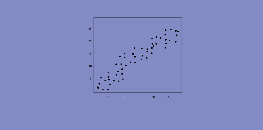
Machine learning has taken the world by storm in recent years. It powers many applications we use every day, from Netflix recommendations to spam email filtering. At its core, machine learning is all about teaching computers to learn and make predictions from data without being explicitly programmed.

One of the most fundamental and widely used machine learning techniques is linear regression. If you‘re new to machine learning, linear regression is a great place to start. In this post, we‘ll cover everything you need to know to understand linear regression and start applying it to real-world problems.

What is Machine Learning?

Before diving into linear regression, let‘s take a step back and define what machine learning is. Machine learning is a subfield of artificial intelligence focused on enabling computers to learn and improve from experience without being explicitly programmed. Machine learning algorithms build models based on sample data in order to make predictions on new data.

There are three main types of machine learning:

1. Supervised learning: The algorithm learns from labeled training data and makes predictions on new unseen data. Examples include spam email classification and housing price prediction.

2. Unsupervised learning: The algorithm finds hidden patterns and structures in unlabeled data. Examples include customer segmentation and anomaly detection.

3. Reinforcement learning: The algorithm learns through interaction with an environment by receiving rewards or punishments. Examples include game playing and robotics.

Linear regression falls under the category of supervised learning, as we use labeled data (with input features and a corresponding output) to train the model to make predictions on new data.

Introduction to Linear Regression

Linear regression is one of the most basic yet powerful machine learning algorithms. It is used for predicting a quantitative response Y based on one or more predictor variables X. At its core, linear regression finds the "best fit" line through the training data that minimizes the differences between the predicted and actual values.

The equation for a simple linear regression with one predictor variable is:

Y = β0 + β1X + ε

Where:

• Y is the response variable
• X is the predictor variable
• β0 is the y-intercept (value of Y when X=0)
• β1 is the coefficient or slope (change in Y per unit change in X)
• ε is the error term

In the case of multiple linear regression with more than one predictor variable, the equation generalizes to:

Y = β0 + β1X1 + β2X2 + … + βpXp + ε

The goal is to find the optimal values of the coefficients (β0, β1, β2, etc.) that minimize the sum of the squared residuals between the actual and predicted Y values. This is typically done using an optimization algorithm like gradient descent.

Assumptions of Linear Regression

For a linear regression model to be valid and unbiased, it needs to satisfy these key assumptions:

1. Linearity: The relationship between X and Y should be linear. This can be checked visually using scatterplots.

2. Independence: The errors should be independent and not correlated with each other. Techniques like the Durbin-Watson statistic can test for correlation of errors.

3. Homoscedasticity: The variance of errors should be constant across all levels of X. Plotting residuals vs fitted values can check for heteroscedasticity.

4. Normality: The errors should be normally distributed with a mean of 0. Q-Q plots or residual histograms can verify normality.

5. No multicollinearity: The predictor variables should not be highly correlated with each other. Variance inflation factor (VIF) is used to detect multicollinearity.

If these assumptions are violated, the model may give misleading results. However, linear regression is considered fairly robust to minor violations of the assumptions.

Evaluating Linear Regression Models

Once we train a linear regression model, how do we know if it‘s any good? Here are some common evaluation metrics:

1. R-squared (coefficient of determination): Measures the proportion of variance in Y that is predictable from X. Values range from 0 to 1, with higher values indicating a better fit. Be cautious of models with high R-squared but poor predictive power (overfitting).

2. Adjusted R-squared: Adjusts R-squared to account for the number of predictor variables. Always lower than regular R-squared. Useful for comparing models with different numbers of predictors.

3. Mean squared error (MSE): Measures the average squared difference between the predicted and actual values. Smaller values are better.

4. Root mean squared error (RMSE): The square root of MSE. Has the same unit as the response variable, making it more interpretable than MSE. Smaller values are better.

It‘s important to evaluate the model on an independent test set that was not used during training to get an unbiased estimate of real-world performance. Cross-validation techniques like k-fold are also commonly used.

Implementing Linear Regression in Python

Let‘s walk through a simple example of training and evaluating a linear regression model using the popular scikit-learn library in Python.

We‘ll use the built-in Boston Housing dataset which contains data on housing prices in the Boston area. The goal is to predict the median value of owner-occupied homes (MEDV) based on variables like the crime rate, number of rooms, age of the property, etc.

from sklearn.datasets import load_boston
from sklearn.linear_model import LinearRegression
from sklearn.model_selection import train_test_split
from sklearn.metrics import mean_squared_error, r2_score

# Load the Boston housing dataset
boston = load_boston()
X = boston.data
y = boston.target

# Split into training and testing sets
X_train, X_test, y_train, y_test = train_test_split(X, y, test_size=0.2, random_state=42)

# Create a linear regression model
model = LinearRegression()

# Train the model
model.fit(X_train, y_train)

# Make predictions on the test set
y_pred = model.predict(X_test)

# Evaluate performance
mse = mean_squared_error(y_test, y_pred)
rmse = np.sqrt(mse)
r2 = r2_score(y_test, y_pred)

print(f"Mean squared error: {mse:.2f}")
print(f"Root mean squared error: {rmse:.2f}")
print(f"R-squared: {r2:.2f}")

Output:

Mean squared error: 25.64
Root mean squared error: 5.06
R-squared: 0.66

Our simple linear regression model achieves an R-squared of 0.66 on the test set, meaning it explains 66% of the variance in housing prices. The RMSE of $5,060 tells us that on average, the model‘s predictions are off by about $5,060. Not too bad for a first attempt!

There are many ways we could improve this model, such as:

• Perform feature selection to remove irrelevant variables
• Engineer new features
• Handle outliers and missing values
• Try alternative regression algorithms (polynomial regression, decision trees, etc.)

Conclusion

We covered a lot of ground in this post, including:

• The fundamentals of machine learning and where linear regression fits in
• How linear regression works under the hood
• The assumptions linear regression makes about the data
• Metrics for evaluating linear regression models
• Implementing linear regression in Python with scikit-learn

Linear regression is a powerful yet simple algorithm that every aspiring machine learning practitioner should have in their toolkit. It‘s widely used for forecasting sales, analyzing customer data, predicting stock prices, and much more.

Some key takeaways:

• Linear regression is best suited for predicting a quantitative output based on one or more quantitative input features
• Always check the assumptions before applying linear regression
• Regression is sensitive to outliers, so be sure to identify and handle them appropriately
• Plotting the data and residuals is a great way to diagnose issues visually
• Don‘t blindly chase a high R-squared – always use your domain knowledge to sanity check the results

I hope this post gave you a solid foundation in linear regression and the confidence to start applying it to your own datasets. Stay curious and never stop learning!