Understanding Conditional Probability and Bayes‘ Theorem: An AI and ML Perspective

Introduction

As an AI and machine learning expert, I cannot overstate the importance of probability theory in our field. Probability provides the mathematical foundation for quantifying and reasoning about the uncertainty inherent in real-world data and decision making. Two of the most fundamental concepts in probability that every AI practitioner must deeply understand are conditional probability and Bayes‘ Theorem.

These concepts are not just theoretical curiosities – they directly underpin and enable many of the most widely used machine learning algorithms and techniques. From Naive Bayes classifiers to Bayesian neural networks, from handling missing data to model selection, conditional probability and Bayes‘ Theorem are everywhere in modern AI.

In this in-depth guide, we‘ll explore these concepts from an AI and ML perspective. We‘ll start with a refresher on the basics, then dive into the many ways conditional probability and Bayes‘ Theorem are applied in machine learning. Along the way, we‘ll look at concrete examples, key ML techniques, and real-world applications. Whether you‘re an AI researcher, ML engineer, or data scientist, by the end of this guide you‘ll have a solid grasp of these essential concepts and how to wield them in your work.

Conditional Probability Recap

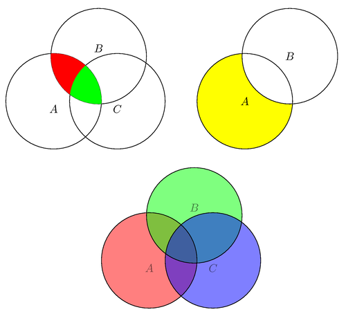
Before we jump into the AI applications, let‘s quickly review what conditional probability is and how to calculate it. Recall that the conditional probability of an event A given event B, denoted as P(A|B), is the probability that event A occurs given that we know event B has occurred. Mathematically:

P(A|B) = P(A ∩ B) / P(B)

where P(A ∩ B) is the probability of the intersection of A and B (i.e., the probability that both events occur), and P(B) is the probability of event B.

A classic example is a medical test for a disease. Let‘s say the test has a 98% true positive rate (sensitivity) and a 97% true negative rate (specificity). The disease prevalence in the population is 1%. If a person tests positive, what is the probability they actually have the disease?

Let D be the event that the person has the disease, and + be the event of a positive test. We are asked to find P(D|+), which we can calculate using Bayes‘ Theorem (derived from the definition of conditional probability):

P(D|+) = P(+|D) P(D) / P(+)
= 0.98 0.01 / (0.98 0.01 + 0.03 0.99)
≈ 0.25

So even with a highly accurate test, the probability of actually having the disease given a positive result is only about 25%! This is because the low prevalence of the disease means there will be many more false positives than true positives. This kind of reasoning is crucial in many AI applications, as we‘ll see next.

Conditional Probability in Machine Learning Evaluation

One of the most immediate applications of conditional probability in machine learning is in model evaluation. Many of the standard metrics used to assess the performance of classification models are based on conditional probabilities.

Consider a binary classification problem, like spam email detection. A confusion matrix summarizes the model‘s performance:

	Actual Spam	Actual Not Spam
Predicted Spam	True Positive (TP)	False Positive (FP)
Predicted Not Spam	False Negative (FN)	True Negative (TN)

Several key metrics can be calculated from the confusion matrix:

• Accuracy = (TP + TN) / (TP + TN + FP + FN)
• Precision (aka Positive Predictive Value) = TP / (TP + FP)
• Recall (aka Sensitivity, True Positive Rate) = TP / (TP + FN)
• Specificity (aka True Negative Rate) = TN / (TN + FP)

Notice that precision and recall are both conditional probabilities! Precision is the probability that an email is actually spam given that the model predicted it as spam. Recall is the probability that the model will predict an email as spam given that it is actually spam.

Here‘s an example confusion matrix:

	Actual Spam	Actual Not Spam
Predicted Spam	90	10
Predicted Not Spam	5	9895

The precision of this spam classifier is:

Precision = 90 / (90 + 10) = 0.90

The recall is:

Recall = 90 / (90 + 5) ≈ 0.947

So 90% of the emails flagged as spam are truly spam, and the model catches 94.7% of all actual spam emails.

The choice of metric depends on the problem. For spam detection, high precision is important to avoid filtering out legitimate emails. For medical diagnosis, high recall is crucial to avoid missing cases of the disease.

Understanding these metrics as conditional probabilities helps interpret their meaning and select the appropriate one for a given application. It also helps guide efforts to improve the model. For example, if precision is low, the model needs to reduce false positives. If recall is low, it needs to reduce false negatives.

Naive Bayes Classifiers

One of the most direct applications of conditional probability in machine learning is the Naive Bayes family of classifiers. These are simple probabilistic classifiers based on applying Bayes‘ Theorem with strong independence assumptions between the features.

Despite their simplicity, Naive Bayes classifiers have proven effective in many real-world situations, particularly in text classification and spam filtering. They require relatively little training data to estimate the necessary parameters.

The "naive" in their name stems from the bold assumption that the features (e.g., the words in a document) are conditionally independent given the class (e.g., spam or not spam). While this assumption is rarely true in reality, Naive Bayes classifiers often still perform surprisingly well.

Mathematically, a Naive Bayes classifier calculates the probability of a class Ck given a feature vector X = (x1, …, xn) using Bayes‘ Theorem:

P(Ck | x1, …, xn) = (P(Ck) * ∏i P(xi | Ck)) / P(x1, …, xn)

The naive independence assumption allows us to write P(x1, …, xn | Ck) = ∏i P(xi | Ck).

In practice, there are several variants of Naive Bayes classifiers depending on the assumed distribution of P(xi | Ck). For example:

• Gaussian Naive Bayes assumes continuous features follow a Gaussian (normal) distribution.
• Multinomial Naive Bayes is common for discrete features, like word counts in text classification.
• Bernoulli Naive Bayes assumes binary features, indicating the presence or absence of the feature.

Here‘s a simple example of using Naive Bayes for text classification in Python using scikit-learn:

from sklearn.naive_bayes import MultinomialNB
from sklearn.feature_extraction.text import CountVectorizer

# Training data
train_text = ["spam spam", "ham ham", "spam ham", "ham spam"]  
train_labels = [1, 0, 1, 0]  # 1 = spam, 0 = ham

# Testing data
test_text = ["spam spam", "ham ham ham"]

# Vectorize text data
vectorizer = CountVectorizer()
train_features = vectorizer.fit_transform(train_text)
test_features = vectorizer.transform(test_text)

# Train Naive Bayes classifier
classifier = MultinomialNB()
classifier.fit(train_features, train_labels)

# Make predictions
predictions = classifier.predict(test_features)
print(predictions)  # Output: [1 0]

This example demonstrates the basic process:

1. Vectorize the text data into numerical features (word counts).
2. Train the Naive Bayes classifier on the feature vectors and corresponding labels.
3. Use the trained classifier to make predictions on new data.

The classifier correctly predicts that "spam spam" is spam (1) and "ham ham ham" is ham (0).

Naive Bayes classifiers are just one example of how conditional probability and Bayes‘ Theorem are directly applied in machine learning algorithms. The same principles underlie more sophisticated techniques like Bayesian networks and Bayesian inference in probabilistic graphical models.

Bayesian vs Frequentist Approaches in Machine Learning

The application of Bayes‘ Theorem in machine learning goes beyond specific algorithms. It represents a fundamentally different way of thinking about probability and uncertainty compared to the traditional frequentist approach.

In the frequentist paradigm, probabilities are interpreted as long-run frequencies of events. Parameters of a model (e.g., weights in a neural network) are considered fixed, unknown constants. The goal is typically to find the single "best" estimate of the parameters, such as the maximum likelihood estimate (MLE) or maximum a posteriori (MAP) estimate.

In contrast, the Bayesian paradigm treats probabilities as degrees of belief about events. Parameters are treated as random variables with their own probability distributions, representing our uncertainty about their true values. The goal is to compute the full posterior distribution of the parameters given the observed data.

Here are some key differences in how these paradigms approach common machine learning tasks:

• Parameter Estimation:

  • Frequentist: Find the single best estimate (e.g., MLE, MAP).
  • Bayesian: Compute the full posterior distribution of the parameters.

• Model Selection:

  • Frequentist: Use criteria like cross-validation error, AIC, BIC.
  • Bayesian: Use Bayesian model evidence, Bayes factors.

• Overfitting:

  • Frequentist: Controlled by regularization, early stopping, etc.
  • Bayesian: Automatically controlled by integrating over parameter uncertainties.

• Uncertainty Quantification:

  • Frequentist: Difficult, relies on approximate techniques like bootstrapping.
  • Bayesian: Naturally quantified in the posterior distributions.

In recent years, there has been growing interest in Bayesian approaches to deep learning. Techniques like variational inference allow approximating the posterior distributions of neural network weights. This enables quantifying the uncertainty in the model‘s predictions, which is crucial for applications like autonomous driving and medical diagnosis where knowing what a model doesn‘t know can be as important as what it does.

That said, Bayesian methods can be computationally expensive, often requiring approximate inference techniques. Frequentist approaches remain prevalent and effective for many tasks. The best approach often depends on the specific problem and available computational resources.

Real-World Applications

The principles of conditional probability and Bayesian inference find use in numerous real-world AI systems. Here are a few examples:

• Recommendation Systems: Online platforms like Netflix and Amazon use probabilistic models to infer user preferences based on their activity. Conditional probabilities help estimate the likelihood a user will enjoy a particular item given their history.

• Autonomous Vehicles: Self-driving cars must constantly make decisions under uncertainty. Bayesian methods allow quantifying and propagating uncertainty from sensor data through the decision-making pipeline.

• Medical Diagnosis: Probabilistic reasoning is essential in medical contexts, from interpreting test results to predicting patient outcomes. Bayesian networks can model complex dependencies between symptoms, risk factors, and diseases.

• Spam Filtering: As we saw, Naive Bayes classifiers are a popular choice for spam detection. More advanced Bayesian techniques can catch more sophisticated forms of spam while minimizing false positives.

• Natural Language Processing: Many NLP tasks, like sentiment analysis and topic modeling, rely on probabilistic models of text. Bayesian approaches allow incorporating prior knowledge and quantifying uncertainty in model outputs.

These are just a few examples – the applications are virtually endless. As AI systems tackle increasingly complex and high-stakes tasks, the ability to reason about uncertainty using the tools of probability becomes ever more critical.

Conclusion

In this guide, we‘ve taken a deep dive into conditional probability and Bayes‘ Theorem from the perspective of an AI and machine learning expert. We‘ve seen how these concepts provide a mathematical foundation for reasoning about uncertainty in data and models.

We explored practical applications, from evaluating classifier performance to the inner workings of Naive Bayes models. We also discussed the broader philosophical divide between Bayesian and frequentist approaches in machine learning, and the growing impact of Bayesian methods in areas like deep learning and uncertainty quantification.

Throughout, we‘ve emphasized the real-world relevance of these ideas with examples drawn from diverse domains like spam filtering, medical diagnosis, and autonomous vehicles. The ubiquity of these applications underscores the importance of a strong grounding in probabilistic thinking for anyone working in AI today.

But beyond the technical details, the Bayesian perspective offers a powerful way of thinking about learning and decision-making under uncertainty. It provides a principled framework for incorporating prior knowledge, updating beliefs in light of new evidence, and quantifying the uncertainty in our conclusions.

As the field of AI continues to advance and grapple with ever more complex and consequential problems, these ideas will only become more central. The most impactful work will be done by those who can deftly wield the tools of probability to navigate a world of uncertainty. Mastering conditional probability and Bayes‘ Theorem is a crucial step on that journey.