A Comprehensive Guide to Solving Business Problems with Markov Chains

Markov chains are a cornerstone of modern artificial intelligence and machine learning, with applications spanning natural language processing, speech recognition, bioinformatics, and more. As a data scientist, it‘s crucial to master this foundational technique, both to understand core concepts in AI/ML, and to directly apply Markov chains to challenging business problems.

In this in-depth guide, we‘ll dive deep into the theory and practice of Markov chains, with a focus on solving real-world business cases. We‘ll provide a rigorous mathematical treatment of the core concepts, illustrate the key ideas with concrete examples, and compare Markov chains to alternative modeling approaches. In addition, we‘ll go beyond the basics, covering advanced techniques like hidden Markov models and Markov decision processes, as well as powerful software packages for Markov chain modeling.

Whether you‘re a data scientist, business analyst, or AI/ML engineer, this guide will give you both the conceptual understanding and practical tools to confidently apply Markov chains to high-impact business problems. Let‘s dive in!

Markov Chains: Mathematical Foundations

Before jumping into applications, it‘s important to establish a solid mathematical foundation. Formally, a Markov chain is a stochastic process that satisfies the Markov property: the probability distribution of the next state depends only on the current state, and not on the sequence of states that preceded it. More precisely:

Let ${X_t : t = 0, 1, 2, \dots}$ be a stochastic process that takes on a finite number of possible values (states). The set of possible states is called the state space, denoted by $S = {s_1, s_2, \dots, s_r}$. If for any sequence of times $t_0 < t1 < \dots < t{n-1} < t_n$ and any sequence of states ${x_0, x1, \dots, x{n-1}, xn, x{n+1}} \subset S$, we have:

$$P(X_{t_n} = xn, X{t{n+1}} = x{n+1} \mid X_{t_0} = x0, X{t_1} = x1, \dots, X{t{n-1}} = x{n-1}) = P(X_{t_n} = xn, X{t{n+1}} = x{n+1} \mid X{t{n-1}} = x_{n-1})$$

then ${X_t}$ is a Markov chain.

The Markov property essentially says that the future state of the system depends only on the present state, and not on how we got to the present state. This memoryless property is a strong assumption, but one that holds approximately in many real-world systems.

A Markov chain is characterized by its transition probability matrix $P$, where $P_{ij}$ is the probability of transitioning from state $i$ to state $j$ in one time step:

$$P{ij} = P(X{t+1} = s_j \mid X_t = s_i)$$

The transition matrix has the following properties:

1. $0 \leq P_{ij} \leq 1$ for all $i,j$
2. $\sum{j=1}^r P{ij} = 1$ for all $i$

Given a specification of the states and transition probabilities, we can simulate the evolution of the system over time. Starting from an initial state distribution $\mu_0$, the state distribution after 1 step is:

$$\mu_1 = \mu_0P$$

And more generally, after $n$ steps:

$$\mu_n = \mu_0P^n$$

A key question is whether this process converges to a steady-state distribution as $n \to \infty$. Under certain regularity conditions (irreducibility, aperiodicity), the Convergence Theorem for Markov chains states that there is a unique distribution $\pi$ such that:

$$\lim_{n \to \infty} \mu_0 P^n = \pi \text{ for all } \mu_0$$

Moreover, $\pi$ is the unique non-negative solution to the equations:

$$\pi = \pi P, \quad \sum_{i=1}^r \pi_i = 1$$

In other words, the steady-state distribution $\pi$ is a left eigenvector of the transition matrix with eigenvalue 1. We can find $\pi$ by solving this system of linear equations.

The steady-state distribution provides valuable information about the long-run behavior of the system. It tells us the proportion of time the system spends in each state, independent of the starting state. This has important applications in areas like web navigation analysis, where the steady-state distribution corresponds to the long-run fraction of traffic on each page.

Another important quantity is the expected hitting time from state $i$ to state $j$, denoted $k_{ij}$. This is the expected number of steps to reach state $j$ when starting from state $i$. It can be found by solving the system of linear equations:

$$k{ij} = 1 + \sum{r \neq j} P{ir} k{rj}, \quad k_{jj} = 0$$

Hitting times are useful in applications like customer churn analysis, where we want to know how long a customer is expected to remain with the company before churning.

Transition Matrix Estimation and Properties

In practice, the transition probabilities are usually not known exactly, but must be estimated from data. Given a sequence of state transitions, the maximum likelihood estimate of $P_{ij}$ is:

$$\hat{P}{ij} = \frac{N{ij}}{\sum{k=1}^r N{ik}}$$

where $N_{ij}$ is the number of observed transitions from state $i$ to state $j$.

It‘s important to quantify the uncertainty in these estimates, especially when the amount of data is limited. One approach is to construct a confidence interval for each $P_{ij}$. Under the Central Limit Theorem, an approximate 95% confidence interval is:

$$\hat{P}{ij} \pm 1.96 \sqrt{\frac{\hat{P}{ij} (1 – \hat{P}{ij})}{\sum{k=1}^r N_{ik}}}$$

We can also perform hypothesis tests on the transition probabilities. For example, to test whether $P_{ij} = p^$ for some hypothesized value $p^$, we can use a binomial test:

$$Z = \frac{\hat{P}{ij} – p^}{\sqrt{\frac{p^ (1 – p^*)}{\sum{k=1}^r N_{ik}}}}$$

Under the null hypothesis, $Z$ follows a standard normal distribution.

Similar statistical techniques can be applied to the steady-state distribution and hitting times. These statistical properties are crucial for assessing the reliability of the model and the conclusions drawn from it.

Industry Applications

Markov chains have found widespread application across a range of industries, including:

• Customer analytics: Markov models of customer behavior can predict churn, segment customers based on their browsing/purchase history, and optimize marketing interventions. For example, a telecommunications company could model customers‘ transitions between usage tiers and proactively target high-value customers at risk of leaving.

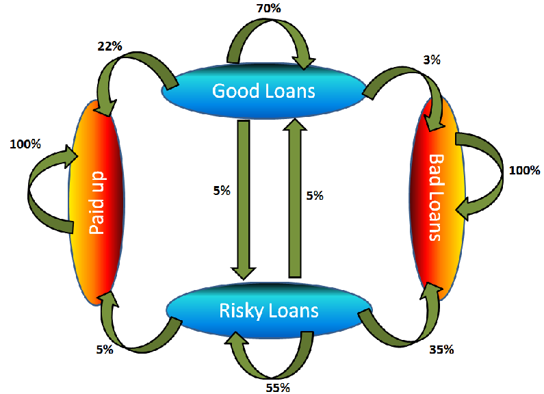
• Financial risk modeling: Markov chains are used extensively in credit risk modeling to capture the dynamics of credit ratings and defaults. A bank could use a Markov model to calculate the probability of a loan transitioning to default over a given time horizon, and set interest rates and capital requirements accordingly.

• Healthcare: Markov models are a standard tool for modeling the progression of chronic diseases, the spread of infections, and the cost-effectiveness of medical interventions. A pharmaceutical company could use a Markov model to evaluate the long-term benefits and risks of a new drug for treating a progressive disease like Alzheimer‘s.

• Operations research: Markov chains can optimize inventory management, queueing systems, and maintenance schedules. For example, a manufacturer could model the deterioration of equipment over time and determine the optimal preventive maintenance policy to minimize downtime and repair costs.

• Web/mobile analytics: Markov models of user navigation can identify common paths through a website or app, predict bounce rates and conversions, and optimize the UI/UX design. An e-commerce company could analyze the clickstream data of visitors using a Markov model and personalize product recommendations to maximize revenue.

The potential applications are endless, but the common theme is that Markov chains provide a principled way to model and predict dynamic systems. By understanding the transition probabilities between states, we can gain deeper insight into the causal mechanisms driving the system and make data-driven decisions to optimize outcomes.

Advanced Techniques and Considerations

While basic Markov chains are already quite powerful, several advanced techniques can extend their capabilities:

• Higher-order Markov chains: In a higher-order Markov chain, the transition probabilities depend on the past $k$ states instead of just the current state. This can capture more long-range dependencies, at the cost of increased model complexity and data requirements. Higher-order Markov chains are commonly used in natural language processing, where the probability of the next word often depends on the previous $k$ words.

• Hidden Markov models: In a hidden Markov model (HMM), the true state of the system is not directly observed, but must be inferred from noisy or incomplete observations. HMMs introduce a separate observation model $P(Y_t \mid X_t)$ describing the probability of observing $Y_t$ given the hidden state $X_t$. The classic application of HMMs is in speech recognition, where the hidden states correspond to phonemes and the observations are acoustic features. The Viterbi and Forward-Backward algorithms can efficiently learn the parameters of an HMM and decode the most likely sequence of hidden states.

• Markov decision processes: A Markov decision process (MDP) models sequential decision-making under uncertainty, where an agent must choose actions to maximize its expected cumulative reward over time. In addition to the transition model $P(X_{t+1} \mid X_t, A_t)$ and observation model $P(Y_t \mid X_t)$, an MDP includes a reward function $R(X_t, A_t)$ specifying the immediate reward for taking action $A_t$ in state $X_t$. The goal is to learn a policy $\pi(A_t \mid X_t)$ mapping states to actions that maximizes the expected long-term reward. Reinforcement learning algorithms like Q-learning can solve MDPs and yield optimal policies. MDPs have been applied to problems like robotic control, autonomous driving, and game playing.

• Continuous-time Markov chains: In a continuous-time Markov chain (CTMC), transitions can occur at any time rather than at discrete time steps. CTMCs are defined by a matrix of transition rates $Q$, where $q{ij}$ is the rate of transitioning from state $i$ to state $j$. The holding time in each state is exponentially distributed with parameter equal to the negative of the diagonal entry $q{ii}$. CTMCs are commonly used to model queues, population dynamics, and reliability systems.

There are also important considerations and limitations to keep in mind when applying Markov chains:

• Assumption validation: The Markov property is a strong assumption that should be validated on a case-by-case basis. In some applications, the future may depend on the distant past, or the transition probabilities may change over time. Residual diagnostics and goodness-of-fit tests can help assess the suitability of a Markov model.

• Data requirements: Estimating the transition matrix requires a large amount of data to get reliable estimates, especially for higher-order chains with many parameters. Insufficient data can lead to overfitting and poor generalization. Regularization techniques like Laplace smoothing can help mitigate this.

• Computational complexity: The time complexity of basic operations on a Markov chain (computing the state distribution, hitting times, steady-state, etc.) scales quadratically with the number of states. For large state spaces, more efficient approximation methods may be necessary, such as Monte Carlo simulation, variational inference, or spectral methods.

• Interpretability: While Markov models are highly interpretable in terms of the transition probabilities and state meanings, this can become more challenging in complex models with many states and higher orders. Careful model selection and visualization techniques are important for maintaining interpretability.

Software and Resources

There are several excellent software packages and libraries for working with Markov chains in Python and R:

• hmmlearn: A Python library for hidden Markov models with support for discrete and Gaussian emissions, Bayesian inference, and model selection.
• PyMC: A Python library for probabilistic programming and Bayesian inference, with built-in support for Markov chain Monte Carlo methods.
• msm: An R package for fitting and analyzing continuous-time Markov chains, with functions for maximum likelihood estimation, model selection, and survival analysis.
• markovchain: An R package for discrete-time Markov chains, with support for simulating and visualizing Markov processes, computing steady-state distributions, and more.

In addition, there are many great resources for learning more about Markov chains and their applications in business and AI/ML:

• "Introduction to Probability Models" by Sheldon Ross – A comprehensive textbook on stochastic models, with in-depth coverage of Markov chains and their properties.
• "Machine Learning: a Probabilistic Perspective" by Kevin Murphy – An authoritative text on machine learning that covers Markov models and related techniques like HMMs and Kalman filters.
• "Probabilistic Graphical Models: Principles and Techniques" by Daphne Koller and Nir Friedman – A seminal work on graphical models, including Markov networks and Bayesian networks, with applications to AI and machine learning.
• "Markov Chains and Mixing Times" by David Levin, Yuval Peres, and Elizabeth Wilmer – A rigorous mathematical treatment of Markov chain convergence and mixing, with applications to MCMC and randomized algorithms.

These resources provide a wealth of knowledge for further exploration and practical application of Markov chains.

Conclusion

In this comprehensive guide, we‘ve explored the theory and practice of using Markov chains to solve real-world business problems. We‘ve covered the mathematical foundations, including the formal definition and key properties of Markov chains, as well as techniques for estimating and validating Markov models from data. We‘ve also seen how Markov chains can be applied across a wide range of industries, from customer analytics to financial risk modeling to healthcare.

Beyond the basics, we‘ve delved into advanced topics like higher-order Markov chains, hidden Markov models, and Markov decision processes, and discussed important considerations and limitations to keep in mind. Finally, we‘ve highlighted powerful software packages and authoritative resources for further learning and application.

Markov chains are a fundamental tool in the data scientist‘s toolkit, providing a principled way to model and predict dynamic systems. By mastering this technique, data scientists and business analysts can unlock valuable insights from sequential data and drive impact across industries. As the fields of artificial intelligence and machine learning continue to advance, Markov chains will undoubtedly remain a core building block for solving challenging problems and pushing the boundaries of what‘s possible.