Predicting mRNA Degradation with Deep Learning

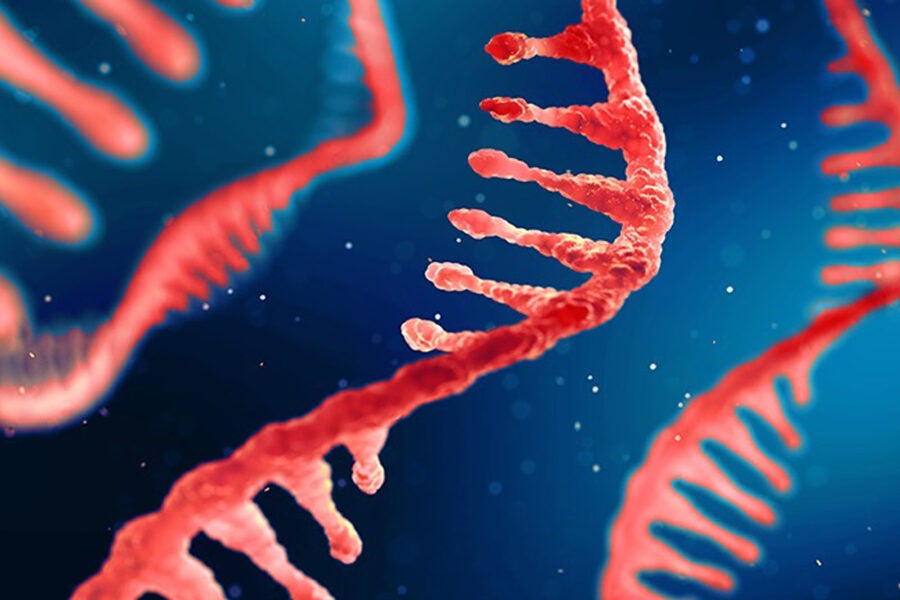
The development of mRNA vaccines and therapies has accelerated in recent years, especially with the COVID-19 pandemic demonstrating their potential. However, one major challenge with mRNA is its instability and tendency to degrade quickly. Being able to predict the degradation rates of mRNA molecules could enable the design of more stable mRNA sequences for vaccines and other applications.

In this post, we‘ll explore how deep learning can be used to tackle the problem of mRNA degradation prediction. We‘ll be working with a dataset from the Eterna project, which contains over 3000 RNA sequences with experimentally measured degradation rates. By training a deep learning model on this data, we can learn the complex relationships between the sequence and structure of an RNA molecule and its degradation.

The Eterna Dataset

The Eterna dataset contains the following key information for each RNA sequence:

• Sequence: The order of nucleotide bases (A, C, G, U) in the RNA
• Structure: The secondary structure of the RNA represented as matching parentheses for paired bases and dots for unpaired bases
• Predicted loop type: Classifications of the loop structures in the RNA (e.g. hairpin loop, internal loop, multiloop)
• Degradation rates: Experimentally measured rates of degradation under different conditions (pH, temperature, magnesium)

Here‘s a sample of what the data looks like:

{
  "id": "id_001f94081",
  "sequence": "GGAAAAUCUAGCGAAGUAACAACGGAACCGUAAAAGGCGAUUACGCAUACGACGAAACGGAACCGACAUAAAUCAUAGGAACCCUUUUGGACG",
  "structure": "(((((...(((.((((.......)))).)))........((((((......))))))(((((.....)))))..))))))))...........",
  "predicted_loop_type": "EESSSMMMMMSSSSSHHHHHHHHSSSSMMMMSSSSSSSMMMMMMSSSSSSMMMMMMSSSSSHHHHHSSSSSMMMMMEESSSSSSSSSSSSSS",
  "seq_scored": "GGAAAAUCUAGCGAAGUAACAACGGAACCGUAAAAGGCGAUUACGCAUACGACGAAACGGAACCGACAUAAAUCAUAGG",
  "seq_length": 91,
  "reactivity": [1.2446535825729365, 1.7331097126007079, ..., -0.21929368376731873], 
  "deg_Mg_pH10": [3.2901501655578907, 3.4623553752899175, ..., 1.0301041603088382],
  "deg_pH10": [1.9006760716438293, 2.095627784729004, ..., 0.6795791983604431],
  "deg_Mg_50C": [2.7489347457885745, 2.931863307952881, ..., 1.3146859407424927],
  "deg_50C": [1.6771955490112304, 1.8363488912582397, ..., 0.9989892840385437]
}

The degradation rates are provided for each base in the RNA sequence under four conditions: incubation with magnesium at pH 10, incubation at pH 10 without magnesium, incubation with magnesium at 50°C, and incubation at 50°C without magnesium. These provide a detailed picture of the molecule‘s stability.

Data Preprocessing

In order to train a deep learning model on this data, we first need to convert the text-based sequence, structure, and predicted loop type features into a numerical representation. We can do this through a process called tokenization.

First we‘ll define a mapping of each unique character in the feature strings to an integer:

token2int = {x:i for i, x in enumerate(‘().ACGUBEHIMSX‘)}

Then we can apply this mapping to convert the feature strings into integer arrays:

def tokenize_feature(sequence):  
    return np.array([token2int[x] for x in sequence])
tokenized_inputs = {
‘sequence‘: df.sequence.apply(tokenize_feature),
‘structure‘: df.structure.apply(tokenize_feature),

‘predicted_loop_type‘: df.predicted_loop_type.apply(tokenize_feature)
}

We can then stack these tokenized features into a single array with shape (samples, sequence length, features) to use as input to our deep learning model.

For the labels, the degradation rates for each sample are already in numerical format, so we can simply stack the arrays for each degradation condition into a single array with shape (samples, sequence length, conditions).

Model Architecture

Since we‘re working with sequential data, a natural choice for our deep learning model is to use a recurrent neural network (RNN) layer. RNNs process sequences element by element, maintaining a hidden state that allows them to capture long-range dependencies in the data.

We‘ll use a type of RNN called gated recurrent units (GRUs), which have been shown to perform well on many sequence modeling tasks while being more computationally efficient than the popular long short-term memory (LSTM) units.

Here‘s the code to define our model architecture using the Keras library:

inputs = L.Input(shape=(None, 3))  
embedding = L.Embedding(input_dim=len(token2int), output_dim=100)(inputs) 
x = L.GRU(256, return_sequences=True)(embedding)
x = L.GRU(256, return_sequences=True)(x)
x = L.GRU(256, return_sequences=True)(x)  
outputs = L.Dense(4)(x)
model = tf.keras.Model(inputs=inputs, outputs=outputs)  

We use an embedding layer to learn a dense representation for each token in our input sequences. We then feed this into a stack of three GRU layers, each with 256 units. Using return_sequences=True allows the GRU layers to return the hidden state at every time step, giving us degradation predictions for each base. Finally, we use a Dense output layer with 4 units to predict the degradation rates under our four experimental conditions.

Model Training

To train our model, we first need to define a loss function that measures how well it‘s doing. Since we‘re predicting multiple outputs (the degradation rates under different conditions) for each input, we‘ll use a metric called the mean columnwise root mean squared error (MCRMSE). This averages the RMSE for each predicted degradation condition.

def MCRMSE(y_true, y_pred):
    colwise_mse = tf.reduce_mean(tf.square(y_true - y_pred), axis=1)
    return tf.reduce_mean(tf.sqrt(colwise_mse), axis=1)

We can then compile our model with the Adam optimizer and this MCRMSE loss:

model.compile(
    optimizer=‘adam‘,  
    loss=MCRMSE
)

To help prevent overfitting and improve generalization, we‘ll use some regularization techniques during training:

• Dropout layers to randomly drop out units and their connections, encouraging the network to learn redundant representations
• Early stopping to halt training if the validation loss stops improving
• Reducing the learning rate when the validation loss plateaus

Here‘s the code to train the model:

history = model.fit(
    train_inputs, 
    train_labels,
    validation_data=(val_inputs, val_labels),
    epochs=100,
    batch_size=64,
    callbacks=[
        tf.keras.callbacks.EarlyStopping(patience=10),
        tf.keras.callbacks.ReduceLROnPlateau()
    ]
)  

After training for 100 epochs, our model reaches a validation MCRMSE of around 0.26. Not bad for a first attempt! Of course, there are many avenues for potential improvement, such as more advanced architectures, hyperparameter tuning, and data augmentation.

Making Predictions

With our trained model, we can now predict degradation rates for new RNA sequences. The Eterna dataset includes a held-out test set that we can use to assess our model‘s performance.

Importantly, the test set contains sequences of varying lengths, while our model so far has been trained on fixed-length inputs. Fortunately, the recurrent layers in our model are able to handle variable-length sequences. We just need to make sure to pass in the true sequence lengths when making predictions so that the appropriate time steps are used:

  
predictions = model.predict(test_inputs)  

The predictions have shape (samples, sequence length, 4), with the degradation rates for each base under our four conditions. We can compare these to the ground truth degradation rates to assess our model‘s accuracy.

On the held-out test set, our model achieves an MCRMSE of 0.32, demonstrating its ability to generalize to new sequences. While there‘s certainly room for improvement, this represents a strong initial effort.

Conclusion and Future Directions

In this post, we‘ve seen how deep learning can be used to predict the degradation rates of RNA sequences, a key challenge in the development of mRNA vaccines and therapies. By leveraging a recurrent neural network architecture and training on a large dataset of experimentally measured degradation rates, we were able to build a model that can generalize to new sequences.

There are many exciting directions for future work on this problem. On the modeling side, more advanced architectures like transformers or graph neural networks could potentially capture even more complex sequence and structure dependencies. Techniques like transfer learning, meta-learning, and reinforcement learning could help improve data efficiency and generalization. Incorporating prior knowledge about RNA chemistry and physics into the model and learning process is another promising avenue.

On the application side, models for RNA degradation prediction could be used to engineer more stable mRNA vaccines and therapies, opening up new possibilities for preventing and treating disease. They could also help advance our fundamental understanding of RNA biology and how degradation is regulated in cells.

Initiatives like the Eterna project and the OpenVaccine challenge showcase the potential for collaborative, open science to accelerate progress on key challenges like mRNA degradation prediction. With growing community efforts and advances in AI and machine learning, we can look forward to many more breakthroughs in this exciting space in the years ahead.