A Detailed Guide to Bayesian Decision Theory – Part 2

Introduction

Welcome back to our in-depth exploration of Bayesian decision theory. In part 1, we laid the groundwork by discussing key concepts like Bayes‘ theorem, prior and posterior probabilities, and how to make classification decisions based on posterior probabilities.

Now, in part 2, we‘ll take things to the next level by generalizing the theory to handle a wider range of real-world scenarios. Buckle up as we dive into feature vectors, loss functions, risk minimization, and more. By the end, you‘ll have a solid grasp of how to apply Bayesian techniques to complex decision-making problems.

Generalizing Bayesian Decision Theory

To make Bayesian decision theory more widely applicable, we‘ll expand our assumptions in four key ways:

1. Allow multiple features instead of just one
2. Handle more than two classes or states of nature
3. Consider actions beyond simple classification, like the option to reject a decision if we‘re unsure
4. Use loss functions to assign different costs to different types of errors

Let‘s unpack each of these in more detail.

From Scalar to Vector: Moving to Feature Space

In part 1, we worked with a single feature x to make our decisions. But most real classification problems involve multiple features. For example, in medical diagnosis, we might consider a patient‘s age, blood pressure, lab results, and symptoms to determine their condition.

To handle multiple features, we move from the scalar value x to a d-dimensional feature vector x in Euclidean space R^d. This space defined by the feature vectors is called the feature space. It‘s a key construct that will come up repeatedly as we generalize the theory.

Expanding the State Space

Previously, we limited ourselves to binary decisions between two states of nature or classes, w1 and w2. But we can expand this to any number of classes w1, w2, …, wc. This will require some new notation but makes the theory more useful. For instance, a self-driving car‘s vision system might need to distinguish between dozens of objects like cars, trucks, signs, pedestrians, etc.

To Classify or Not to Classify? Introducing Rejection

Up to now, we‘ve assumed that our decision-maker must assign the input to one of the known classes. But in some cases, the wise choice may be to not decide at all! This is known as rejection.

Rejection can be the best option when:

• The input is ambiguous and assigning it to any class is prone to error
• Making an incorrect decision is very costly
• We have the option to gather more information instead of deciding now

Bayesian decision theory handles rejection by broadening the set of possible actions. In addition to actions corresponding to each class (decide w1, decide w2, etc.), we introduce a "reject" action. The theory will guide us on when to choose it.

Not All Errors Are Equal: Introducing Loss Functions

In binary classification, we usually assume that false positives and false negatives are equally bad. But that‘s often not the case. Think of medical diagnosis, where a false negative (failing to detect a serious condition) is generally worse than a false positive (thinking a healthy patient is sick).

Loss functions allow us to specify different costs for different kinds of mistakes. The loss λ(αi |wj) is the penalty for taking action αi (e.g. deciding class i) when the true class is wj.

We‘ll see how loss functions fit into the overall decision-making framework shortly. But first, we need to define a few more key concepts.

Posterior Probabilities and Conditional Risk

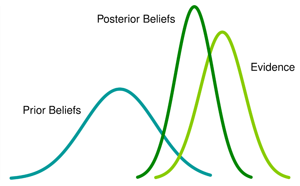
Recall from part 1 that Bayes‘ theorem allows us to calculate the posterior probability P(wj|x) – the probability that the true class is wj given that we‘ve observed feature vector x. It states:

P(wj|x) = p(x|wj) P(wj) / p(x)

where P(wj) is the prior probability of class wj, p(x|wj) is the likelihood of observing x given class wj, and p(x) is the evidence – the total probability of observing x across all classes.

We can calculate the evidence by summing the numerator over all c classes:

p(x) = ∑_{j=1}^c p(x|wj) P(wj)

Once we have the posterior probabilities, we can define the conditional risk R(αi|x) – the expected loss of taking action αi given that we observed x:

R(αi|x) = ∑_{j=1}^c λ(αi|wj) P(wj|x)

In words, to find the risk of action αi, we sum the products of the loss and posterior probability for each possible class. Intuitively, this captures the average loss we‘d incur by always taking action αi when we see x, averaged over the different possible true classes.

Finding the Optimal Decision Rule

We now have the tools to state the goal of Bayesian decision theory formally: find the decision rule α(x) that minimizes the overall risk.

Remember that a decision rule is a function that maps each possible feature vector x to one of the actions α1, α2, …, αa. The overall risk R of a decision rule is:

R = ∫ R(α(x)|x) p(x) dx

This intimidating-looking equation is actually quite intuitive: to calculate the overall risk, we integrate the conditional risk R(α(x)|x) over the entire feature space, weighted by the probability p(x) of observing each x.

To minimize R, we simply choose the action that minimizes the conditional risk at each x. In other words, for each x, we evaluate R(αi|x) for i=1, …, a and select the αi that yields the smallest value. This gives us our optimal decision rule α(x).

The minimum overall risk achieved by this optimal decision rule is called the Bayes risk. It represents the best possible performance we can achieve given the limitations of our data and assumptions.

Two-Class Example

To solidify these concepts, let‘s walk through a two-class example. We have classes w1 and w2, and actions α1 (decide w1) and α2 (decide w2).

The loss function is defined by four values:

• λ11 = λ(α1|w1) = loss of deciding w1 when true class is w1
• λ12 = λ(α1|w2) = loss of deciding w1 when true class is w2
• λ21 = λ(α2|w1) = loss of deciding w2 when true class is w1
• λ22 = λ(α2|w2) = loss of deciding w2 when true class is w2

The conditional risks are:

R(α1|x) = λ11 P(w1|x) + λ12 P(w2|x)
R(α2|x) = λ21 P(w1|x) + λ22 P(w2|x)

To find the optimal decision rule, we choose α1 if R(α1|x) < R(α2|x), and α2 otherwise.

Working through the math, this condition simplifies to:

p(x|w1) / p(x|w2) > (λ12 – λ22) P(w2) / (λ21 – λ11) P(w1)

The left side is the likelihood ratio – the relative probability of observing x under each class. The right side is a threshold that depends on the loss values and prior probabilities.

So our decision rule boils down to: pick class w1 if the likelihood ratio exceeds a fixed threshold, and w2 otherwise. This is called the likelihood ratio test, and it crops up frequently in Bayesian analysis.

Worked Example

Let‘s apply what we‘ve learned to a toy dataset:

         Sample No              Width               Height              Class                

1 Small Small C1
2 Medium Small C2
3 Medium Large C2
4 Large Small C1
5 Medium Medium C1
6 Large Large C1
7 Small Medium C2
8 Large Medium C1

1. First, let‘s calculate the prior probabilities P(w1) and P(w2).

There are 5 samples in class C1 and 3 in C2, so:

P(C1) = 5/8 = 0.625
P(C2) = 3/8 = 0.375

2. Now, suppose we observe a new sample with features (Small, Large). Which class should we assign it to?

To decide, we calculate the posterior probabilities P(C1|Small, Large) and P(C2|Small, Large) using Bayes‘ rule:

P(C1|Small, Large) = p(Small, Large|C1) P(C1) / p(Small, Large)

P(C2|Small, Large) = p(Small, Large|C2) P(C2) / p(Small, Large)

To evaluate these, we need the likelihoods p(Small, Large|C1) and p(Small, Large|C2).

From the data, we see that:

• In class C1, 0 out of 5 samples have (Small, Large). So p(Small, Large|C1) = 0/5 = 0.
• In class C2, 0 out of 3 samples have (Small, Large). So p(Small, Large|C2) = 0/3 = 0.

Plugging in the numbers:

P(C1|Small, Large) = 0 * 0.625 / p(Small, Large) = 0

P(C2|Small, Large) = 0 * 0.375 / p(Small, Large) = 0

Uh oh, both posteriors are zero! This is because our tiny dataset doesn‘t contain any examples of (Small, Large). In practice, we‘d gather more data or apply smoothing techniques to avoid zero probabilities.

But for now, let‘s arbitrarily choose class C2 since it has lower prior probability. This aligns with the principle of picking the least likely class when we‘re maximally uncertain.

3. Finally, what‘s the probability that we misclassified this sample?

Well, since we chose class C2, the probability of error is just the probability that the sample actually belongs to C1:

P(error) = P(C1|Small, Large) = 0

In this case, we‘re certain about our choice (for better or worse). With a larger, more representative dataset, we‘d likely have non-zero posteriors and some chance of being wrong.

Real-World Applications

Bayesian decision theory isn‘t just an academic exercise – it powers many real-world systems. Here are a few examples:

• Medical diagnosis: Doctors use Bayesian reasoning to combine disease prevalence (priors) with patient symptoms and test results (likelihoods) to determine the most likely diagnosis (posteriors).

• Spam filters: Email services employ Naive Bayes classifiers (a simplification of Bayesian decision theory) to decide whether incoming messages are spam or ham based on their word frequencies.

• Document categorization: Similar Bayesian techniques can automatically sort news articles, web pages, or scientific papers into predefined topics based on their text content.

• Machine learning: Many modern ML algorithms, from simple linear regression to advanced deep learning models, can be interpreted through a Bayesian lens. The Bayesian perspective provides a principled way to incorporate prior knowledge and quantify uncertainty.

Conclusion

Whew, that was quite the journey! Let‘s recap what we‘ve learned in this two-part series:

• Bayesian decision theory provides a principled framework for making optimal decisions under uncertainty by combining prior knowledge with observed data.
• The key ingredients are prior probabilities, likelihoods, loss functions, and posterior probabilities, related by Bayes‘ famous theorem.
• To handle realistic problems, we can generalize the theory to work with feature vectors, multiple classes, rejection actions, and arbitrary loss functions.
• The optimal Bayesian decision rule selects the action that minimizes conditional risk for each possible observation. This rule also minimizes the overall risk and achieves the lowest possible Bayes risk.

Of course, we‘ve only scratched the surface of this rich and fascinating field. To dive deeper, check out these excellent resources:

• Pattern Classification by Duda, Hart, and Stork – the classic textbook on statistical pattern recognition and Bayesian decision theory

• Machine Learning: A Probabilistic Perspective by Kevin Murphy – a comprehensive guide to Bayesian machine learning techniques

• Seeing Theory – an interactive visual introduction to Bayesian inference and decision-making

I hope this series has demystified Bayesian decision theory and shown you its power and elegance. While the math may seem daunting at first, the core ideas are quite intuitive. With a little practice (and a lot of data), you‘ll be making optimal decisions like a pro!

As always, if you have any questions or want to share your own insights, don‘t hesitate to reach out. Until next time, happy deciding!