A Deep Dive into Bayesian Decision Theory: Discriminant Functions for Normal Densities

1. Introduction

Welcome back to our in-depth series on Bayesian decision theory! In the previous articles, we laid the groundwork by discussing the fundamentals of Bayesian decision making, discriminant functions, decision surfaces, and the multivariate normal distribution. Armed with this knowledge, we‘re now ready to tackle the core topic of this post: deriving and analyzing the discriminant functions for normally distributed features.

Buckle up, because we‘re about to embark on a mathematical journey through the realm of discriminant analysis. By the end of this article, you‘ll have a solid grasp of how to perform Bayesian classification when dealing with Gaussian data. Let‘s dive in!

2. A Quick Recap

Before we get into the nitty-gritty details, let‘s briefly review some key concepts from our previous discussions:

• In Bayesian decision theory, our goal is to minimize the expected loss (or risk) by choosing the class that maximizes the posterior probability P(ωi|x).
• Rather than working directly with the posterior, it‘s often more convenient to use a discriminant function gi(x) that preserves the same decision rule. The optimal class is the one with the highest discriminant score.
• For multivariate normal densities, the discriminant function takes the following form:

gi(x) = −(1/2)(x−μi)^T Σi^(−1) (x−μi) − (d/2)ln(2π) − (1/2)ln(|Σi|) + ln(P(ωi))

where μi and Σi are the mean vector and covariance matrix for class ωi, and d is the number of features.

3. Case 1: Independent Features with Equal Variances

Let‘s start with the simplest scenario, where the features are statistically independent and have the same variance σ^2 for all classes. In this case, the covariance matrix Σi is reduced to a diagonal matrix σ^2I, where I is the identity matrix.

Plugging this into our generic discriminant function and ignoring the terms that are independent of the class index i, we obtain the following:

gi(x) = −(1/2σ^2) ||x−μi||^2 + ln(P(ωi))

Here, ||x−μi||^2 represents the squared Euclidean distance between the feature vector x and the class mean μi. Intuitively, this discriminant function favors classes whose mean is closer to the observed data point, while also taking into account the prior probabilities P(ωi).

We can further expand the equation and drop the quadratic term x^Tx that appears in all gi(x). This leads us to the equivalent linear discriminant function:

gi(x) = w_i^T x + w_i0

where w_i = (1/σ^2)μi and w_i0 = −(1/2σ^2)μi^Tμi + ln(P(ωi)).

The resulting decision boundaries are linear hyperplanes defined by gi(x) = gj(x). If the prior probabilities are equal, the hyperplane is simply the perpendicular bisector of the line segment connecting the class means. Otherwise, it is shifted towards the less likely class.

The figure above illustrates how the decision boundary adapts to different prior probabilities in a two-dimensional feature space. When the priors are equal (left), the boundary lies halfway between the means. As one class becomes more likely (right), the boundary moves closer to the other class to compensate.

4. Case 2: Equal Covariance Matrices

Now let‘s consider a slightly more general situation where the covariance matrices are the same for all classes, i.e., Σi = Σ. Although less common in practice, this case provides a nice bridge between the independent features assumption and the fully general setting.

Starting from the multivariate normal discriminant function and dropping the irrelevant terms, we arrive at:

gi(x) = −(1/2)(x−μi)^T Σ^(−1) (x−μi) + ln(P(ωi))

If the prior probabilities are equal, the decision rule simplifies to choosing the class with the nearest mean vector, where distance is measured using the Mahalanobis metric induced by Σ^(−1).

As before, we can expand the quadratic form and discard the x^T Σ^(−1) x term to obtain a linear discriminant:

gi(x) = w_i^T x + w_i0

where w_i = Σ^(−1)μi and w_i0 = −(1/2)μi^T Σ^(−1)μi + ln(P(ωi)).

The decision boundary between classes ωi and ωj is a hyperplane defined by:

w^T(x−x0) = 0

where
w = Σ^(−1)(μi−μj)
x0 = (1/2)(μi+μj) − (ln(P(ωi)/P(ωj))/(μi−μj)^T Σ^(−1) (μi−μj))(μi−μj).

Unlike Case 1, the hyperplane is not necessarily orthogonal to the line connecting the means, and it doesn‘t pass through the midpoint unless the priors are equal. The direction of the hyperplane depends on the shape of the shared covariance matrix.

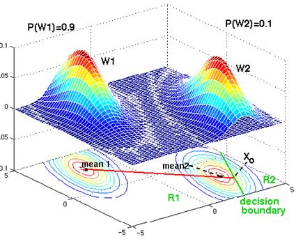
In the figure above, we see how the decision boundary is affected by both the covariance matrix (which determines the orientation of the elliptical contours) and the prior probabilities (which control the amount of shift from the midpoint).

5. Case 3: Arbitrary Covariance Matrices

Finally, we arrive at the most general and realistic scenario, where each class has its own covariance matrix Σi. In this setting, the discriminant function retains its quadratic form:

gi(x) = −(1/2)(x−μi)^T Σi^(−1) (x−μi) − (1/2)ln(|Σi|) + ln(P(ωi))

Expanding the quadratic term, we can rewrite this as:

gi(x) = x^T W_i x + w_i^T x + w_i0

where
W_i = −(1/2)Σi^(−1)
w_i = Σi^(−1)μi
w_i0 = −(1/2)μi^T Σi^(−1)μi − (1/2)ln(|Σi|) + ln(P(ωi)).

The decision boundaries between classes are now quadratic surfaces (hyperquadrics) rather than hyperplanes. These surfaces can take on various shapes depending on the relative magnitudes and orientations of the covariance matrices, including hyperboloids, paraboloids, ellipsoids, and even more exotic forms.

The figure showcases the rich variety of decision boundaries that can occur when the covariance matrices are distinct. The specific geometry is determined by the interplay between the shapes, sizes, and orientations of the class-conditional densities.

6. Practical Considerations

While the theoretical foundations of discriminant analysis are relatively straightforward, there are several practical issues to keep in mind when applying these techniques to real-world problems:

• Estimating parameters: In most cases, the true class means and covariances are unknown and must be estimated from training data. The maximum likelihood estimates are simply the sample means and covariances. However, these estimates can be unreliable when the training set is small relative to the number of features, leading to overfitting. Regularization techniques like shrinkage or dimensionality reduction may be necessary.

• Choosing priors: The prior probabilities P(ωi) can have a significant impact on the decision boundaries, especially when the classes are not well-separated. If the true priors are known (e.g., from domain knowledge), they should be used. Otherwise, they can be estimated from the training set proportions or treated as tuning parameters.

• Handling class imbalance: When the classes have very different frequencies, the learned decision boundaries may be skewed towards the majority class. This can lead to poor performance on the minority class(es). Strategies for dealing with imbalanced data include oversampling the minority class, undersampling the majority class, or adjusting the misclassification costs.

• Assessing assumptions: Discriminant analysis relies on the assumption that the class-conditional densities are multivariate normal. If this assumption is violated, the resulting decision boundaries may be suboptimal or misleading. It‘s important to check the normality of the data (e.g., using Q-Q plots or hypothesis tests) and consider alternative models if necessary.

• Computational complexity: The time and space complexity of discriminant analysis grows with the number of features d and the number of classes k. In the general case (QDA), inverting the covariance matrices takes O(d^3) time. With high-dimensional data, this can be prohibitively expensive. Dimensionality reduction techniques like PCA can help alleviate this burden.

7. Applications and Examples

Discriminant analysis has been successfully applied in a wide range of domains, including:

• Face recognition: LDA can be used to extract discriminative features from face images and classify them into different categories (e.g., individuals, emotions, attributes).

• Document classification: By representing documents as word frequency vectors, QDA can be employed to automatically categorize them by topic, sentiment, or authorship.

• Genomic data analysis: Discriminant analysis is a popular tool for identifying genetic markers that are predictive of disease risk or treatment response.

• Sensor fusion: In applications like robotics and autonomous driving, discriminant functions can be used to integrate data from multiple sensors (e.g., cameras, lidars, radars) and make robust decisions.

Here‘s a simple example of how to perform LDA using Python‘s scikit-learn library:

from sklearn.datasets import load_iris
from sklearn.discriminant_analysis import LinearDiscriminantAnalysis

# Load the iris dataset
iris = load_iris()
X, y = iris.data, iris.target

# Fit the LDA model
lda = LinearDiscriminantAnalysis()
lda.fit(X, y)

# Predict the class labels for new data points
X_new = [[5.0, 3.5, 1.3, 0.3], 
         [6.6, 3.0, 4.4, 1.4]]
y_pred = lda.predict(X_new)

print(y_pred)  # Output: [0 1]

This code snippet demonstrates how to train an LDA model on the classic iris flower dataset and use it to classify new samples. The resulting predictions indicate that the first sample belongs to class 0 (setosa) and the second belongs to class 1 (versicolor).

For a more in-depth treatment of discriminant analysis and other classification algorithms, I recommend checking out the following resources:

• The Elements of Statistical Learning by Hastie, Tibshirani, and Friedman
• Pattern Recognition and Machine Learning by Christopher Bishop
• scikit-learn documentation on LDA and QDA

8. Conclusion

In this article, we took a deep dive into the discriminant functions for multivariate normal densities and explored their behavior under different assumptions about the covariance structure. We saw how the decision boundaries can range from simple linear hyperplanes to complex quadratic surfaces, depending on the degree of flexibility allowed in the model.

Along the way, we discussed some of the practical challenges that arise when applying discriminant analysis to real-world problems, including parameter estimation, model selection, and computational scalability. We also highlighted a few concrete examples of how these techniques are used in various application domains.

At its core, discriminant analysis is a powerful and versatile framework for probabilistic classification that leverages the elegant properties of the Gaussian distribution. By providing a principled way to incorporate prior knowledge and make optimal decisions in the face of uncertainty, it remains a fundamental tool in the machine learning and statistics toolbox.

Of course, there‘s much more to be said about discriminant analysis and its extensions, such as regularized discriminant analysis, kernel discriminant analysis, and subspace discriminant analysis. But I hope this article has given you a solid foundation to build upon and sparked your curiosity to learn more.

As always, thank you for reading, and happy learning!