A Comprehensive Guide to DBSCAN Clustering: How It Works, Parameter Tuning, and Python Implementation

Introduction

Clustering is an essential unsupervised machine learning technique for discovering hidden patterns and structures in data. While popular algorithms like K-means and hierarchical clustering are widely used, they have limitations in detecting clusters of arbitrary shapes and handling noisy data. This is where DBSCAN (Density-Based Spatial Clustering of Applications with Noise) shines as a powerful density-based clustering algorithm.

In this in-depth guide, we‘ll dive into the inner workings of DBSCAN, understand its key concepts and parameters, learn how to implement it in Python, and explore its advantages, limitations, and applications. Whether you‘re a beginner or an experienced practitioner, this article will equip you with the knowledge to leverage DBSCAN effectively in your clustering tasks. Let‘s get started!

What is DBSCAN Clustering?

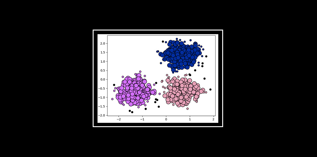
DBSCAN is a density-based clustering algorithm that groups together data points that are closely packed, marking points in low-density regions as outliers or noise. Unlike K-means, which requires specifying the number of clusters upfront, DBSCAN automatically determines the number of clusters based on the density of the data.

The key idea behind DBSCAN is that clusters are dense regions in the data space, separated by regions of lower density. It defines clusters as connected dense regions and is able to identify clusters of arbitrary shapes, making it versatile for various data distributions.

How DBSCAN Works

To understand how DBSCAN works, let‘s familiarize ourselves with its key concepts:

1. Core Points: A data point is considered a core point if it has at least a specified number of neighboring points (min_samples) within a specified radius (epsilon).

2. Border Points: A data point that is not a core point but falls within the epsilon radius of a core point is called a border point.

3. Noise Points: A data point that is neither a core point nor a border point is considered a noise point or an outlier.

4. Directly Density-Reachable: A point q is directly density-reachable from a core point p if it is within the epsilon radius of p.

5. Density-Reachable: A point q is density-reachable from a point p if there is a chain of directly density-reachable points connecting p to q.

6. Density-Connected: Two points p and q are density-connected if there exists a point o such that both p and q are density-reachable from o.

DBSCAN starts by selecting an arbitrary unvisited point in the dataset. If this point is a core point (has at least min_samples neighbors within epsilon radius), it starts a new cluster and expands it by iteratively adding directly density-reachable points. If the point is a border point, it is assigned to the cluster of its core point. If the point is a noise point, it is marked as noise and the algorithm moves on to the next unvisited point.

The algorithm repeats this process until all points in the dataset have been visited. The result is a set of clusters and noise points.

DBSCAN Parameters: Epsilon and Min_Samples

DBSCAN requires two key parameters:

1. Epsilon (eps): The radius of the neighborhood around a point. It determines the maximum distance between two points for them to be considered neighbors.

2. Min_Samples: The minimum number of points required in the epsilon neighborhood of a point for it to be considered a core point.

Choosing appropriate values for these parameters is crucial for the performance of DBSCAN. A small epsilon may result in many small clusters and noise points, while a large epsilon may merge distinct clusters. Similarly, a low min_samples value may classify many points as core points, while a high value may miss sparse clusters.

One approach to select epsilon is by using a k-distance graph. For each point, the distance to its kth nearest neighbor is plotted. The optimal epsilon value is often chosen as the elbow point in this graph, where the distance starts to increase rapidly.

DBSCAN Algorithm Steps

Here‘s a step-by-step breakdown of the DBSCAN algorithm:

1. Select an unvisited point p in the dataset.
2. Retrieve all points density-reachable from p within epsilon radius.
3. If the number of neighboring points is greater than or equal to min_samples, mark p as a core point and start a new cluster. Assign all neighboring points to this cluster.
4. Iterate through each point q in the cluster:
   • If q is unvisited, retrieve its epsilon neighborhood.
   • If the number of neighboring points is greater than or equal to min_samples, add those points to the cluster.
5. Continue expanding the cluster until no more points can be added.
6. If p is a border point (not a core point), assign it to the cluster of its core point.
7. If p is a noise point (neither core nor border), mark it as noise.
8. Repeat steps 1-7 until all points in the dataset have been visited.

Advantages and Disadvantages of DBSCAN

Advantages:

• Automatically determines the number of clusters based on data density.
• Can identify clusters of arbitrary shapes and sizes.
• Robust to outliers and noise points.
• Does not require specifying the number of clusters upfront.

Disadvantages:

• Sensitive to the choice of epsilon and min_samples parameters.
• May struggle with datasets of varying densities.
• Not suitable for high-dimensional data due to the curse of dimensionality.
• Output may change with the order of processing points.

Implementing DBSCAN in Python with scikit-learn

Let‘s see how to implement DBSCAN clustering in Python using the scikit-learn library. Here‘s an example code snippet:

from sklearn.cluster import DBSCAN
from sklearn.datasets import make_moons

# Generate sample data
X, _ = make_moons(n_samples=200, noise=0.05, random_state=42)

# Create DBSCAN object
dbscan = DBSCAN(eps=0.3, min_samples=5)

# Fit the model
dbscan.fit(X)

# Get cluster labels
labels = dbscan.labels_

# Plot the clusters
plt.scatter(X[:, 0], X[:, 1], c=labels, cmap=‘viridis‘)
plt.xlabel(‘Feature 1‘)
plt.ylabel(‘Feature 2‘)
plt.title(‘DBSCAN Clustering‘)
plt.show()

In this example, we generate sample data using the make_moons function from scikit-learn. We create a DBSCAN object with eps=0.3 and min_samples=5. We then fit the model to the data using the fit method and obtain the cluster labels using dbscan.labels_. Finally, we visualize the clusters using a scatter plot.

Advanced Topics: HDBSCAN

While DBSCAN is a powerful clustering algorithm, it has limitations in handling datasets with varying densities. HDBSCAN (Hierarchical Density-Based Spatial Clustering of Applications with Noise) is an extension of DBSCAN that addresses this issue.

HDBSCAN builds a hierarchy of clusters by varying the epsilon parameter and extracts the most stable clusters from this hierarchy. It can handle datasets with varying densities and provides a more robust clustering solution.

The key advantages of HDBSCAN over DBSCAN are:

• Ability to handle datasets with varying densities.
• Automatic selection of the number of clusters.
• Provides a hierarchical clustering structure.
• More robust to parameter settings.

Applications and Use Cases of DBSCAN

DBSCAN clustering finds applications in various domains, including:

1. Anomaly Detection: DBSCAN can identify outliers or anomalies in data as noise points that do not belong to any cluster.

2. Image Segmentation: DBSCAN can segment images into regions based on pixel density and connectivity.

3. Geographic Data Analysis: DBSCAN is suitable for clustering geographic data points based on their spatial proximity.

4. Social Network Analysis: DBSCAN can identify communities or clusters in social networks based on the density of connections.

5. Bioinformatics: DBSCAN can cluster biological data, such as gene expression profiles or protein sequences, based on their similarity.

Conclusion

In this comprehensive guide, we explored the DBSCAN clustering algorithm in depth. We learned about its key concepts, parameters, and algorithm steps. We discussed its advantages and disadvantages compared to other clustering algorithms like K-means and hierarchical clustering.

We also saw how to implement DBSCAN in Python using scikit-learn and touched upon the advanced HDBSCAN algorithm. Finally, we explored some common applications and use cases of DBSCAN in various domains.

DBSCAN is a powerful density-based clustering algorithm that can automatically determine the number of clusters, handle arbitrary cluster shapes, and identify noise points. By understanding its inner workings and parameter tuning techniques, you can effectively apply DBSCAN to your clustering tasks and uncover meaningful patterns in your data.

Remember to experiment with different parameter settings, visualize your results, and validate the clusters using domain knowledge. With DBSCAN in your toolkit, you‘re well-equipped to tackle a wide range of clustering challenges and gain valuable insights from your data.

Happy clustering!