Mastering Markov Chains: A Comprehensive Guide with R

Introduction

Markov chains are a fundamental concept in probability theory and a workhorse of modern machine learning, underlying everything from natural language processing and recommender systems to financial modeling and reinforcement learning. Despite their ubiquity and power, Markov chains remain a mystery to many data scientists and developers. In this in-depth guide, we‘ll unpack the mathematical theory behind Markov chains, explore their applications in AI/ML, and show you how to implement them efficiently in R.

Whether you‘re a veteran data scientist looking to refresh your probability chops or a beginner seeking to add a versatile tool to your modeling arsenal, this article will equip you with the knowledge and code to tackle real-world problems with Markov chains. Buckle up and let‘s dive in!

Formal Definition

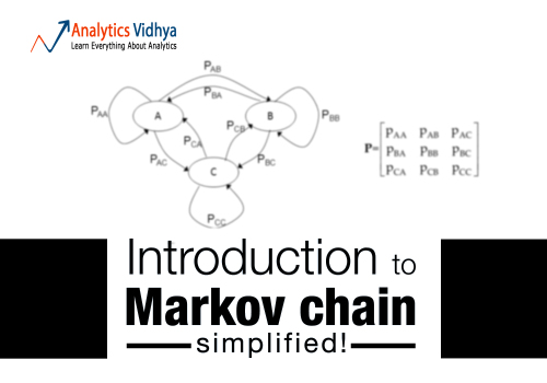
A Markov chain is a stochastic process that satisfies the Markov property – the probability distribution of the next state depends only on the current state, not the full history. More formally, let {X_t : t = 0, 1, 2, …} be a sequence of random variables taking values in some countable set S (the state space). The process is a Markov chain if:

P(X_t+1 = j | X_t = i, X_t-1 = k, …) = P(X_t+1 = j | X_t = i) = p_ij

for all t ≥ 0 and i, j, k ∈ S. The probabilities {p_ij : i, j ∈ S} are called the transition probabilities and form the entries of the transition matrix P, where P[i,j] = p_ij.

A Markov chain is homogeneous if the transition probabilities p_ij are independent of t. We‘ll focus on homogeneous chains for the rest of this article.

Memory and Higher-Order Chains

The defining characteristic of a Markov chain is its memoryless property – the next state depends only on the current state, not the history. However, we can extend this to consider higher-order dependencies.

In an m-th order Markov chain, the next state depends on the previous m states:

P(X_t+1 = x_t+1 | X_t = x_t, …, X₁ = x₁) = P(X_t+1 = x_t+1 | X_t = x_t, …, X_t-m+1 = x_t-m+1)

For example, in a 2nd-order chain, the probability of the next word in a sentence depends on the previous two words, capturing more context. Higher-order chains can model more complex dependencies but suffer from the curse of dimensionality, as the number of parameters grows exponentially with the order.

Applications in Machine Learning

Reinforcement Learning

Markov chains form the backbone of many reinforcement learning (RL) algorithms. In RL, an agent learns to make sequential decisions by interacting with an environment modeled as a Markov decision process (MDP). An MDP is an extension of a Markov chain that includes actions and rewards.

The goal is to learn a policy π(a|s) – a mapping from states to action probabilities – that maximizes the expected cumulative reward. Many RL algorithms, such as policy iteration and value iteration, exploit the Markov property to efficiently estimate value functions and optimize policies.

Text Generation

Markov chains are a simple yet effective approach to generating realistic text sequences. By training a Markov chain on a corpus of sentences or characters, we can learn transition probabilities between words or characters. To generate new text, we sample from the learned distributions, producing sequences that mimic the style and structure of the training data.

For example, a character-level Markov chain trained on Shakespeare‘s works might generate passages like:

"To be, or not to be, that is the question:
Whether ‘tis nobler in the mind to suffer
The slings and arrows of outrageous fortune,
Or to take arms against a sea of troubles,
And by opposing end them?"

While not perfectly coherent, the model captures some of Shakespeare‘s distinctive language patterns. Higher-order Markov chains and more sophisticated language models like recurrent neural networks can generate even more convincing text.

Music Generation

Similar to text, we can use Markov chains to generate new musical sequences by learning transition probabilities between notes or chords. This is the basis of many algorithmic composition systems and generative music apps.

By training separate Markov chains on different musical styles or composers, we can create mashups and novel combinations. We can also condition the transitions on additional variables like tempo and instrumentation for finer control.

Here‘s a simple example of a melody generator using R‘s markovchain package:

library(markovchain)

notes <- c("C", "D", "E", "F", "G", "A", "B")
durations <- c("whole", "half", "quarter", "eighth")

# Define transition matrices
note_trans <- matrix(c(
  0.2, 0.2, 0.2, 0.1, 0.1, 0.1, 0.1,
  0.1, 0.2, 0.2, 0.2, 0.1, 0.1, 0.1,
  0.1, 0.1, 0.2, 0.2, 0.2, 0.1, 0.1,
  0.1, 0.1, 0.1, 0.2, 0.2, 0.2, 0.1,
  0.1, 0.1, 0.1, 0.1, 0.2, 0.2, 0.2,
  0.2, 0.1, 0.1, 0.1, 0.1, 0.2, 0.2,
  0.2, 0.2, 0.1, 0.1, 0.1, 0.1, 0.2), 
  nrow = 7, byrow = TRUE, dimnames = list(notes, notes)  
)

duration_trans <- matrix(c(
  0.4, 0.3, 0.2, 0.1,
  0.3, 0.4, 0.2, 0.1,
  0.2, 0.3, 0.4, 0.1, 
  0.1, 0.1, 0.3, 0.5),
  nrow = 4, byrow = TRUE, dimnames = list(durations, durations)
)

# Create Markov chains
note_mc <- new("markovchain", transitionMatrix = note_trans, states = notes)
duration_mc <- new("markovchain", transitionMatrix = duration_trans, states = durations)  

# Generate a 20-note melody
melody <- rmarkovchain(n = 20, object = note_mc, t0 = "C")
durations <- rmarkovchain(n = 20, object = duration_mc, t0 = "half")

print(paste(melody, durations))

This generates a sequence of notes and durations like:

[1] "C half"     "C quarter"  "A eighth"   "F quarter"  "C quarter"  "D half"    
[7] "E half"     "G quarter"  "F half"     "E quarter"  "C quarter"  "F quarter" 
[13] "G quarter"  "F half"     "G quarter"  "C quarter"  "A quarter"  "F eighth"  
[19] "C quarter"  "D quarter" 

Of course, this is a simplistic example – in practice, we would want to train on a larger dataset of melodies, enforce more structural constraints, and use more musically meaningful state representations. But it illustrates the core idea of using Markov chains to capture stylistic patterns and generate new sequences.

Simulation and Sampling

Markov chains provide a powerful tool for sampling from complex, high-dimensional probability distributions. The key idea is to construct a Markov chain whose stationary distribution π equals (or approximates) the target distribution p(x) we want to sample from.

Then, by running the chain for a sufficient number of steps, we can generate samples from p(x) without explicitly computing it. This is the basis of Markov chain Monte Carlo (MCMC) methods, a cornerstone of Bayesian inference and probabilistic machine learning.

Two of the most popular MCMC algorithms are Metropolis-Hastings and Gibbs sampling:

• Metropolis-Hastings: At each step, propose a new state x‘ according to a proposal distribution q(x‘|x), and accept or reject it based on the ratio p(x‘)/p(x). This ensures the chain converges to the target distribution.

• Gibbs sampling: For multivariate distributions, update each variable in turn by sampling from its conditional distribution given the current values of all other variables. This is often more efficient than Metropolis-Hastings for high-dimensional problems.

Here‘s a simple implementation of Metropolis-Hastings in R to sample from a bimodal Gaussian mixture distribution:

target_dist <- function(x) {
  0.3*dnorm(x, mean = -2, sd = 1) + 0.7*dnorm(x, mean = 2, sd = 0.5)
}

metropolis_hastings <- function(n_samples, proposal_sd) {
  samples <- numeric(n_samples)
  current <- 0

  for (i in 1:n_samples) {
    proposal <- current + rnorm(1, sd = proposal_sd)
    accept_prob <- min(1, target_dist(proposal) / target_dist(current))

    if (runif(1) < accept_prob) {
      current <- proposal
    }

    samples[i] <- current
  }

  samples
}

samples <- metropolis_hastings(n_samples = 10000, proposal_sd = 1)

hist(samples, breaks = 50, main = "Metropolis-Hastings Sampling",
     xlab = "x", ylab = "Frequency", xlim = c(-5, 5))

This generates a histogram of samples that approximates the true bimodal distribution:

MCMC is an incredibly rich and active area of research, with numerous variations and extensions. Markov chains provide the mathematical foundation for these powerful sampling techniques.

Convergence and Mixing

A crucial question when working with Markov chains is whether they will converge to a unique stationary distribution π, and how quickly. The stationary distribution is a fixed point of the transition matrix:

π = π P

A sufficient condition for a unique stationary distribution is that the chain is irreducible (it‘s possible to get from any state to any other) and aperiodic (the return times to each state are not deterministic). Such chains are called ergodic.

The mixing time of a Markov chain quantifies how fast it converges to its stationary distribution. This depends on the spectral gap – the difference between the two largest eigenvalues of the transition matrix. Chains with larger spectral gaps mix faster.

In practice, we often run a Markov chain for a burn-in period to reach its stationary distribution, and then collect samples. Diagnostic tests like the Gelman-Rubin statistic can check if multiple chains have converged to the same distribution.

Understanding convergence and mixing properties is crucial for designing efficient Markov chain samplers and ensuring the validity of results.

Conclusion

We‘ve covered a lot of ground in this whirlwind tour of Markov chains, from their basic definition and properties to advanced applications in machine learning. We‘ve seen how Markov chains can model sequences, generate text and music, and enable efficient sampling from complex distributions.

The beauty of Markov chains lies in their simplicity and flexibility – by specifying a set of states and transition rules, we can capture the essential dynamics of countless real-world systems. At the same time, the theory of Markov chains is rich and deep, with connections to linear algebra, graph theory, and optimization.

While we‘ve focused on discrete-time, homogeneous Markov chains in this article, there are many extensions and variations worth exploring – continuous-time chains, hidden Markov models, semi-Markov processes, and more. Markov chains also have close ties to other models like recurrent neural networks and dynamic Bayesian networks.

Whether you‘re analyzing customer behavior, generating creative content, or building the next AlphaGo, Markov chains are a powerful addition to any data scientist‘s toolbox. I hope this article has demystified some of the core concepts and sparked your curiosity to dive deeper. Happy modeling!