Reducing Data Complexity with Variable Clustering: A Guide for SAS and Python Users

Introduction

In the era of big data, analysts and data scientists routinely encounter high-dimensional datasets with hundreds or even thousands of variables. While more data can be a blessing, it often comes with a host of challenges. High dimensionality can drastically increase computation times, introduce redundancy and noise, and make it difficult to explore relationships between variables.

Fortunately, a variety of dimensionality reduction techniques exist to help condense and simplify such datasets while preserving the most important information. In this post, we‘ll dive into one powerful method – variable clustering – and demonstrate how to implement it from scratch using SAS and Python.

What is Variable Clustering?

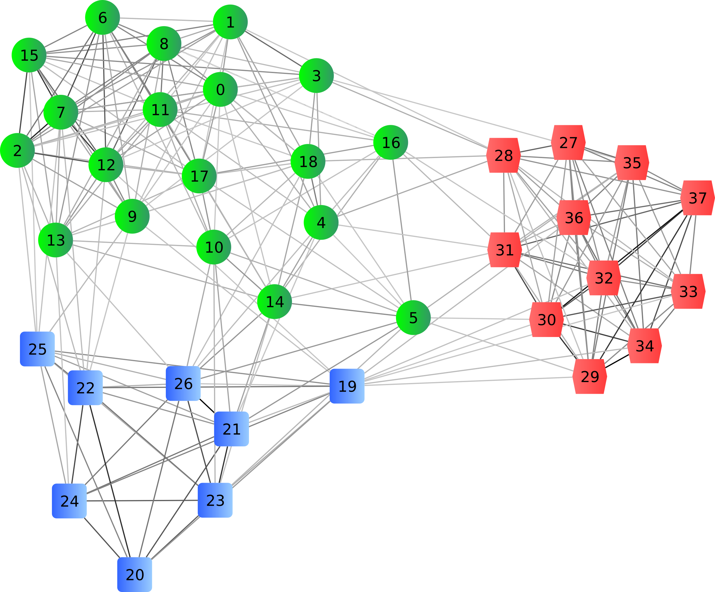
Variable clustering is an unsupervised learning technique that seeks to group similar variables together based on their correlations. The goal is to partition a set of variables into distinct clusters, where variables within a cluster are highly correlated with each other but not with variables in other clusters.

Once the clusters are formed, a single representative variable is selected from each one, while the remaining variables in the cluster are dropped. This has the effect of reducing the total number of variables in the dataset (potentially by a large margin) while still capturing most of the original information. The selected variables can then be used in downstream analysis and modeling.

Under the Hood: How Variable Clustering Works

At the heart of the variable clustering methodology is principal component analysis (PCA). PCA is a technique for deriving a set of new uncorrelated variables, called principal components, from the original possibly correlated variables. These principal components are linear combinations of the original variables, and are derived in decreasing order of the amount of variance they explain in the data.

To illustrate, let‘s work through a simplified example. Consider the following correlation matrix for 10 variables:

(insert correlation matrix image)

We can calculate the first principal component (PC1) by taking a weighted sum of the original variables. The weights, called factor loadings, are chosen to maximize the variance explained by PC1 while maintaining unit variance. Mathematically, PC1 is calculated as:

PC1 = a1X1 + a2X2 + … + a10*X10

where X1 to X10 are standardized versions of the original variables and the weights a1 to a10 are the factor loadings for PC1.

These loadings can be obtained by summing the rows and columns of the correlation matrix and then dividing the column totals by the square root of the grand total:

(show factor loading calculation steps and final loadings for PC1)

We then calculate the residual correlations by subtracting the outer product of the PC1 loadings from the original correlation matrix. This residual matrix has the PC1 correlations removed.

The same process is then repeated on the residual matrix to obtain the second principal component (PC2), third principal component, and so on, until we have derived weights for all 10 PCs. The amount of variance explained by each PC is captured in its eigenvalue, which is simply the sum of squares of its factor loadings.

Two important by-products of PCA are the eigenvalues for each PC and the communality values for each variable. Communality measures the portion of a variable‘s variance that is explained by all the PCs, and is calculated by summing the squared factor loadings across PCs.

(show table of factor loadings, eigenvalues, and communalities)

Splitting and Selecting

Variable clustering adopts this PCA machinery to determine the optimal grouping of variables. Rather than using principal components for scoring and dimensionality reduction as in standard PCA, variable clustering uses them to decide how to split and select variables.

The algorithm starts with all variables in a single cluster. It then performs PCA and checks the second eigenvalue (that is, the eigenvalue for PC2). If this value exceeds a pre-defined threshold, it indicates there is significant remaining correlation in the data and that the cluster should be split into two. This splitting procedure is performed recursively on the subclusters until no second eigenvalue exceeds the threshold.

Once the final clusters have been determined, the next step is to select a representative variable from each cluster to retain. Intuitively, we want to select the variable that is most correlated with other variables in its own cluster but not with variables in other clusters.

This intuition is formalized in the 1-R^2 ratio, where R^2 represents the coefficient of determination from regressing a variable on the components from its own cluster vs. components from other clusters. The variable with the lowest 1-R^2 ratio in each cluster is selected and the rest are eliminated.

Coding It Up: SAS and Python Implementations

Equipped with an understanding of the core concepts, let‘s see how to translate this into code. We‘ll use a publicly available dataset with 63 mixed-type variables as an example.

In SAS, variable clustering can be performed using the VARCLUS procedure:

proc varclus data=mydata maxeigen=0.7 short;
var var1-var63;
run;

The MAXEIGEN option specifies the threshold for splitting clusters based on the second eigenvalue. The SHORT option limits the output to a more readable summary.

In Python, variable clustering can be implemented using a combination of the sklearn and scipy libraries:

import pandas as pd
from sklearn.decomposition import PCA
from scipy.cluster import hierarchy as hc

data = pd.read_csv(‘mydata.csv‘)

correlations = data.corr()
pca = PCA(n_components=data.shape[1])
pca.fit(correlations)

clusters = hc.fclusterdata(correlations, criterion=‘maxclust‘, t=data.shape[1])

First we calculate the correlation matrix, then fit a PCA model with the number of components equal to the number of variables. This gives us access to the full eigenvalues to assess for splitting. Finally, we use hierarchical clustering to assign cluster labels based on the max number of clusters.

(show final cluster assignments and 1-R^2 ratios in SAS and Python)

Interpreting the Output

The key pieces of information to extract from the variable clustering output are:

1. The number of clusters. This tells you the effective dimensionality reduction achieved. In our example, the original 63 variables were reduced to 40 clusters/variables in Python and 35 in SAS.

2. The cluster assignments and 1-R^2 ratios. This shows which variables were grouped together and which variable was selected from each cluster. Lower 1-R^2 ratios indicate stronger within-cluster correlation.

3. The selected variable list. This is the final subset of variables you would use in place of the originals for downstream applications. Comparing this list to the full variable list gives a sense of the complexity reduction.

While the specific clusters differed slightly between SAS and Python, likely due to differences in algorithms and rounding, the overall number of clusters and selected variables were quite similar.

Things to Keep in Mind

When performing variable clustering, there are a few key considerations and limitations to be aware of:

1. The MAXEIGEN threshold (or number of clusters in Python) controls the granularity of the clustering. Higher thresholds will yield fewer, larger clusters and more dimensionality reduction, but also potentially more information loss. The optimal value depends on the specific data and use case.

2. Variable clustering is not a lossless procedure. Information is necessarily discarded when eliminating variables, so it‘s important to validate that key relationships and structures are preserved in the reduced dataset before proceeding.

3. Variables of different types (continuous, categorical, binary, etc.) can affect the correlations and clustering. It may be necessary to rescale, normalize, or recode variables to make them more comparable.

4. Variable clustering is just one approach to dimensionality reduction. Other techniques like traditional PCA, t-SNE, autoencoders, etc. may be more suitable depending on the data and goals.

Conclusion

High-dimensional data presents many challenges, but variable clustering offers a principled way to reduce complexity while preserving key structures. By grouping similar variables and selecting a representative from each cluster, we can often achieve significant dimensionality reduction with minimal information loss.

The core concepts of PCA, eigenvalues, communality, and 1-R^2 ratios provide the foundation for understanding how variable clustering works. And with modern software like SAS and Python, these concepts are readily translated into code for practical application.

While variable clustering is a powerful tool, it‘s important to keep its limitations and assumptions in mind. It is not a universal solution, but rather one of many dimensionality reduction techniques that may be applied. As always, the specific data and analytical goals should dictate the approach.

Hopefully this post has provided a comprehensive conceptual and practical introduction to variable clustering. Armed with this knowledge, I encourage you to try applying it to your own high-dimensional datasets and seeing the benefits firsthand.