A Comprehensive Guide to Spatial Interpolation: Foundations, Methods, and Future Directions

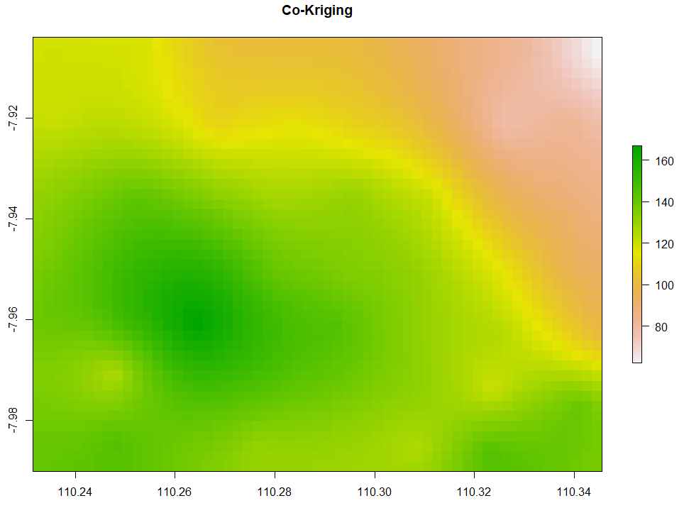
Spatial interpolation is a fundamental tool in geospatial data analysis, enabling estimation of values at unobserved locations based on a set of known measurements. It finds critical applications across diverse fields such as meteorology, oceanography, geology, epidemiology, and environmental science, to name a few. Whether mapping rainfall, air pollution, or soil properties, interpolation empowers us to create continuous surfaces from discrete point data, revealing spatial patterns and enabling further modeling and analysis.

The need for interpolation arises whenever data collection is constrained by logistical factors like cost, time, or accessibility. We may have measurements at weather stations, soil sampling sites, or air quality monitors, but need a complete surface to understand the full spatial context, compute spatial statistics, or feed into other models. Interpolation fills in these gaps, making the most of our available data.

Over the decades, a rich variety of interpolation methods have been developed, each with its own mathematical foundations, assumptions, strengths, and limitations. Some rely solely on the spatial coordinates and measured values, while others leverage additional explanatory variables to guide predictions. Classical methods like inverse distance weighting and kriging have stood the test of time, while newer machine learning techniques like neural networks offer fresh perspectives and capabilities.

In this article, we‘ll take a comprehensive tour of the landscape of spatial interpolation, from the underlying mathematical principles to the state-of-the-art in methods and applications. Code examples in R will demonstrate practical implementation, while visual aids build intuition around the inner workings of each approach. We‘ll discuss how to select an appropriate method for a given problem, and explore the frontiers of research where spatial interpolation intersects with the latest advances in AI and machine learning. Whether you‘re a geospatial data scientist, researcher, or analyst, this guide will equip you with the knowledge and tools to unleash the full power of spatial interpolation in your work.

The Mathematical Foundations of Spatial Interpolation

At its core, spatial interpolation is a problem of function estimation: given a set of observed data points (x_i, y_i), we aim to estimate the value of the function y at any unobserved point x. This is an ill-posed problem, as there are infinitely many functions that could fit the observed data. To make it tractable, we must impose some additional constraints or assumptions about the form of the function or the structure of the spatial data.

Different interpolation methods impose different assumptions and constraints. For example:

• Nearest neighbor assumes the function is piecewise constant, with the value at any point equal to that of the nearest observed data point.
• Inverse distance weighting assumes the function is a weighted average of observed values, with weights inversely proportional to distance.
• Kriging assumes the function is a realization of a Gaussian random field with a specific covariance structure.
• Radial basis functions assume the function is a linear combination of nonlinear basis functions centered at the observed points.

Mathematically, we can express a general interpolation function as:

$\hat{y}(x) = \sum_{i=1}^{n} w_i(x) y_i$

Where $\hat{y}(x)$ is the estimated value at location x, y_i are the observed values, and w_i(x) are the weights assigned to each observed value. The key distinction between methods lies in how these weights are calculated.

For example, in inverse distance weighting, the weights are calculated as:

$w_i(x) = \frac{d(x,xi)^{-p}}{\sum{j=1}^{n} d(x,x_j)^{-p}}$

Where d(x,x_i) is the distance between the prediction point x and the observed point x_i, and p is a power parameter controlling the rate at which influence declines with distance.

In ordinary kriging, the weights are found by solving a system of linear equations that minimize the expected mean squared prediction error, subject to the constraint of unbiasedness. This leads to weights of the form:

$wi(x) = \sum{j=1}^{n} \lambda_j(x) C(x_i,x_j) + \mu(x)$

Where C(x_i,x_j) is the covariance between observed points, $\lambda_j(x)$ are Lagrange multipliers, and $\mu(x)$ is a Lagrange parameter enforcing the unbiasedness constraint.

These mathematical foundations provide a common language for understanding and comparing different interpolation methods. By examining the assumptions implicit in the choice of weight function, we can gain insight into the strengths, limitations, and appropriate use cases for each approach.

A Taxonomy of Interpolation Methods

Interpolation methods can be broadly categorized based on several key characteristics:

1. Deterministic vs. stochastic: Deterministic methods like inverse distance weighting and radial basis functions produce a single predicted surface from the observed data. Stochastic methods like kriging incorporate randomness and yield both predictions and measures of uncertainty.

2. Exact vs. approximate: Exact interpolators like nearest neighbor and inverse distance weighting preserve the observed values at sample locations. Approximate methods like kriging and splines may not honor the observed data exactly in order to produce a smoother surface.

3. Global vs. local: Global methods like polynomial trend surfaces and regression use all available data to make each prediction. Local methods like inverse distance weighting and kriging use only a subset of nearby points.

4. Univariate vs. multivariate: Univariate methods predict a single variable based on its own observed values. Multivariate methods like cokriging and regression kriging incorporate secondary variables to improve predictions.

The table below summarizes some of the key characteristics of popular interpolation methods:

Method	Type	Exact/Approx.	Global/Local	Univar/Multivar
Nearest Neighbor	Deterministic	Exact	Local	Univariate
Inverse Distance Weighting	Deterministic	Exact	Local	Univariate
Radial Basis Functions	Deterministic	Approximate	Global	Univariate
Ordinary Kriging	Stochastic	Approximate	Local	Univariate
Universal Kriging	Stochastic	Approximate	Local	Univariate
Regression Kriging	Stochastic	Approximate	Local	Multivariate
Cokriging	Stochastic	Approximate	Local	Multivariate

This taxonomy provides a useful framework for understanding the relationships between methods and selecting an appropriate approach for a given problem. For example, if preserving the exact observed values is critical, an exact interpolator like nearest neighbor or inverse distance weighting may be preferred. If incorporating secondary information is desired, a multivariate method like regression kriging or cokriging would be a natural choice.

Interpolation and Machine Learning

In recent years, the rapid advances in machine learning have opened up new avenues for spatial interpolation. Many machine learning algorithms, at their core, are fundamentally tools for function approximation – learning complex mappings from input features to output values. This makes them well-suited to the interpolation task, where the goal is to learn a function that maps spatial coordinates (and potentially other covariates) to the variable of interest.

Neural networks, in particular, have shown great promise for spatial interpolation. A neural network is a highly flexible nonlinear function approximator, capable of learning complex patterns and relationships from data. In the context of interpolation, a neural network takes the spatial coordinates (and any other relevant covariates) as inputs, and outputs the predicted value of the target variable.

The structure of a neural network used for interpolation might look something like:

Input Layer (x, y, [covariates]) -> Hidden Layer(s) -> Output Layer (predicted value)

The network is trained on the observed data, learning the weights of the connections between neurons that minimize the prediction error. Once trained, the network can be used to make predictions at any new location.

Some key advantages of neural networks for interpolation include:

• Ability to learn complex, nonlinear relationships between spatial coordinates, covariates, and the target variable
• Flexibility to incorporate a wide variety of input features (e.g., satellite imagery, terrain attributes)
• Scalability to large datasets through mini-batch training and GPU acceleration
• Unified framework for both univariate and multivariate interpolation

Another exciting area of confluence between machine learning and spatial interpolation is Gaussian process regression (GPR). GPR is a powerful Bayesian approach to function estimation that has deep connections to kriging. In fact, under certain conditions, GPR and kriging are mathematically equivalent.

In GPR, the unknown function is modeled as a realization of a Gaussian process – a collection of random variables, any finite number of which have a joint Gaussian distribution. The Gaussian process is fully specified by its mean function and covariance function (kernel). The mean function encodes any prior knowledge about the shape of the function, while the covariance function encodes assumptions about the smoothness and spatial structure.

Given observed data, GPR computes the posterior distribution over functions, which can be used to make predictions at new locations along with uncertainty estimates. Some key benefits of GPR for interpolation are:

• Provides a principled, probabilistic framework for interpolation and uncertainty quantification
• Allows incorporation of prior knowledge through choice of mean and covariance functions
• Enables automatic relevance determination to select important covariates
• Offers a natural way to handle noisy observations and irregular sampling

As an example, here‘s how GPR could be used for interpolation in Python using the scikit-learn library:

from sklearn.gaussian_process import GaussianProcessRegressor
from sklearn.gaussian_process.kernels import RBF, WhiteKernel

# Train GP model
kernel = RBF() + WhiteKernel()
gpr = GaussianProcessRegressor(kernel=kernel, n_restarts_optimizer=10)
gpr.fit(train_coords, train_values)

# Make predictions
pred_means, pred_stds = gpr.predict(test_coords, return_std=True)

The intersection of machine learning and spatial interpolation is a rich and rapidly evolving area of research. As new ML techniques emerge and computational power increases, we can expect to see even more powerful and flexible tools for interpolation in the coming years.

Challenges and Future Directions

Despite the power and sophistication of modern interpolation methods, several key challenges remain:

1. Nonstationarity: Many methods assume that the spatial structure of the data is stationary – that is, the same across the entire study area. However, this is often unrealistic, particularly for large or complex regions. Developing methods that can handle nonstationarity, such as local kriging or geographically weighted regression, is an active area of research.

2. Anisotropy: Interpolation methods often assume that spatial autocorrelation is isotropic – the same in all directions. However, many real-world phenomena exhibit anisotropy, with autocorrelation stronger in some directions than others. Incorporating anisotropy into interpolation models, through tools like directional variograms, is another important challenge.

3. High-dimensional data: With the proliferation of remote sensing and other high-resolution data sources, interpolation problems are increasingly high-dimensional, with many covariates available at each location. Efficiently incorporating this information while avoiding overfitting and maintaining computational tractability is a major challenge. Techniques from machine learning, such as regularization and feature selection, may play a key role here.

4. Uncertainty quantification: While some methods like kriging provide built-in measures of prediction uncertainty, many do not. Developing robust, reliable methods for quantifying uncertainty in interpolated surfaces is crucial for informed decision-making and risk assessment. Bayesian approaches, which treat the unknown surface as a probability distribution, offer a promising avenue for this.

5. Scalability: As data volumes continue to grow, the computational demands of interpolation can become a bottleneck. Developing fast, scalable algorithms that can handle massive datasets is an ongoing challenge. Approaches leveraging parallel computing, GPU acceleration, and approximate methods like variational inference may be key to meeting this challenge.

Looking to the future, we can expect the landscape of spatial interpolation to be shaped by several key trends:

• Increasing integration of machine learning techniques, particularly deep learning and Gaussian processes, into traditional interpolation frameworks
• Greater emphasis on physics-informed interpolation, leveraging knowledge of the underlying processes to constrain and guide predictions
• More flexible, adaptive methods that can automatically detect and adjust to local spatial structure and nonstationarity
• Tighter coupling with GIS and spatial data infrastructure, enabling seamless integration of interpolation into geospatial workflows
• Continued development of open-source software and libraries, making advanced interpolation techniques accessible to a wider audience

As the volume, variety, and velocity of spatial data continue to grow, the importance of effective interpolation will only increase. By understanding the foundations, embracing new techniques from machine learning and statistics, and rising to the challenges outlined above, the geospatial data science community can continue to push the boundaries of what‘s possible with spatial interpolation, unlocking new insights and empowering better decisions in domains from public health to climate change to precision agriculture and beyond.

Conclusion

Spatial interpolation is a vital tool in the geospatial data scientist‘s toolkit, enabling us to turn sparse, irregularly sampled data into rich, continuous surfaces that reveal patterns, inform models, and support decisions. From the simplest nearest neighbor method to the most sophisticated machine learning approaches, interpolation offers a spectrum of techniques to suit a wide range of data types, assumptions, and analysis goals.

As we‘ve seen, each interpolation method is grounded in a set of mathematical principles and assumptions about the nature of spatial data. Understanding these foundations is key to choosing an appropriate method and interpreting the results correctly. But interpolation is not a static field – it‘s constantly evolving, with new techniques from statistics, machine learning, and computational science offering fresh perspectives and capabilities.

To make the most of spatial interpolation, data scientists need a firm grasp of the classical methods, an awareness of the latest developments in AI and machine learning, and a willingness to engage with the challenges at the frontiers of the field. This requires not only technical proficiency, but also a deep understanding of the domain, close collaboration with subject matter experts, and a commitment to rigorous validation and uncertainty quantification.

The potential applications of spatial interpolation are vast, from filling gaps in environmental monitoring networks to creating high-resolution poverty maps to guiding precision agriculture. As the volume and diversity of geospatial data continue to explode, the demand for skilled practitioners who can wield interpolation effectively will only grow.

If you‘re a data scientist looking to expand your geospatial capabilities, investing time to master spatial interpolation is well worth the effort. Start with the basics, experiment with different methods on real data, and don‘t be afraid to dive into the mathematical details. Keep an eye on the latest research, and look for opportunities to apply machine learning techniques to interpolation problems. And above all, remember that interpolation is not a black box – it‘s a tool that requires careful thought, clear communication, and close collaboration with domain experts to yield meaningful, actionable insights.

With the right skills and mindset, spatial interpolation can be a powerful arrow in your quiver, enabling you to extract maximum value from geospatial data and contribute to solving some of the most pressing challenges facing our world today. So dive in, get your hands dirty with data, and start exploring the exciting world of spatial interpolation!