A Beginner‘s Guide to Continuous Probability Distributions for AI and Machine Learning

Probability distributions are the bedrock of machine learning (ML) and artificial intelligence (AI). They provide a language for reasoning about uncertain outcomes, quantifying our beliefs, and making decisions under uncertainty. While discrete probability distributions model variables that take on distinct values, continuous probability distributions are used for variables that can take any value in a range. From sensor readings to pixel intensities to latent representations, continuous variables arise in all areas of AI/ML practice. Having a solid grasp of continuous distributions is crucial for any aspiring AI/ML practitioner.

In this guide, we‘ll introduce the key concepts of continuous probability distributions from the ground up and explore their many applications in modern AI/ML. Whether you‘re a beginner or looking to refresh your knowledge, this article will equip you with the intuition and practical skills to work with continuous distributions in your AI/ML projects. Let‘s dive in!

What are Continuous Probability Distributions?

A continuous probability distribution models a variable that can take any value in a range, limited only by the precision of our measurements. Some examples of continuous variables:

• The height or weight of a person
• The time until an event occurs
• The concentration of a chemical in a solution
• Pixel intensity values in an image
• Latent factors in a recommender system

In contrast to discrete distributions which assign probabilities to distinct outcomes, continuous distributions specify the probability of falling within a range of values. The probability of any exact value is vanishingly small (effectively zero) since there are uncountably infinite values in any range.

Continuous distributions are defined by a mathematical function called the probability density function (PDF), denoted f(x). The PDF specifies the relative likelihood of observing different values of the random variable X. While the PDF can take any non-negative value, the area under the entire PDF curve is always 1, reflecting the fact that the variable must take some value.

To find the probability that X falls in a particular range [a, b], we integrate the PDF over that range:

P(a ≤ X ≤ b) = ∫abf(x)dx

The cumulative distribution function (CDF) of a continuous distribution, denoted F(x), gives the probability that X is less than or equal to a given value x:

F(x) = P(X ≤ x) = ∫-∞xf(t)dt

The CDF is the area under the PDF curve up to the value x. To find the probability of X falling between a and b, we can use the CDF:

P(a < X ≤ b) = F(b) – F(a)

Continuous distributions have several properties that make them mathematically convenient and practically useful:

• They are fully specified by a small number of parameters (like the mean and variance for a normal distribution)
• Many have analytical expressions for the PDF and CDF, enabling efficient computation
• They can be fit to empirical data using techniques like maximum likelihood estimation
• They exhibit useful properties like the Central Limit Theorem and closure under transformations

With this foundation, let‘s meet some of the most important continuous probability distributions and see how they are used in AI and ML.

Common Continuous Probability Distributions in AI/ML

While there are infinitely many possible continuous distributions, a few families arise frequently in AI and ML applications. Here we introduce the key players and their unique properties.

The Normal (Gaussian) Distribution

The crown jewel of continuous distributions, the normal (or Gaussian) distribution is ubiquitous in statistical modeling. It‘s defined by two parameters: the mean μ and the variance σ2, with PDF:

f(x) = (1 / √(2πσ2)) * e^(-((x-μ)^2) / (2σ2))

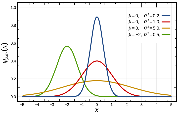
The standard normal distribution sets μ = 0 and σ = 1 and is the basis for many statistical techniques. Some key properties of normal distributions:

• They are symmetric about the mean μ
• 68% of the probability mass falls within 1σ of the mean, 95% within 2σ, and 99.7% within 3σ
• As the number of samples increases, the sampling distribution of the mean becomes approximately normal regardless of the distribution of the population (Central Limit Theorem)

In AI/ML, we frequently assume that noise or errors are normally distributed with zero mean. This simplifies learning algorithms and enables analytical results. Some applications of normal distributions in AI/ML:

• Gaussian naive Bayes for classification
• Gaussian mixture models for clustering and density estimation
• Gaussian processes for regression and optimization
• Variational autoencoders with Gaussian latent variables
• Bayesian inference with Gaussian priors/posteriors

The Exponential Distribution

The exponential distribution models the waiting time until an event occurs, given a constant average rate of occurrence λ. The PDF is:

f(x) = λe^(-λx) for x ≥ 0, 0 otherwise

Properties of the exponential distribution:

• The mean and standard deviation are both 1/λ
• It‘s the continuous analogue of the geometric distribution
• It exhibits the memoryless property: P(X > s + t | X > s) = P(X > t)

In AI/ML, we use the exponential distribution to model inter-arrival times, event occurrences, and survival analysis. It also forms the basis of the Poisson process and is used in models like hidden semi-Markov models.

The Gamma Distribution

The gamma distribution generalizes the exponential to waiting times for the k-th event. It‘s defined by shape k > 0 and rate θ > 0:

f(x) = (θ^k / Γ(k)) x^(k-1) e^(-θx) for x ≥ 0, 0 otherwise

The exponential is a special case when k=1. Key properties:

• Mean is k/θ and variance is k/θ^2
• The sum of exponential random variables follows a gamma distribution
• It‘s the conjugate prior for the rate parameter of the Poisson and exponential

In AI/ML, gamma distributions are used to model waiting times, cluster sizes, and as flexible priors on positive-valued parameters like precision. They also arise in variational inference and to sample from other distributions like the Beta and Dirichlet.

The Multivariate Normal Distribution

Generalizing the normal distribution to multiple variables, the multivariate normal PDF for d-dimensional vector x is:

f(x) = (1 / √((2π)^d |Σ|)) * e^(-1/2 (x-μ)^T Σ^-1 (x-μ))

where μ is the mean vector and Σ is the covariance matrix.

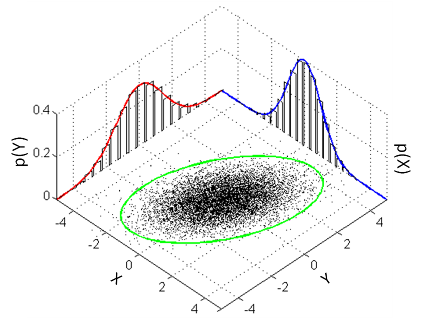
Properties of the multivariate normal:

• Marginal and conditional distributions of subsets of variables are also normal
• Allows for correlation between variables through the covariance matrix
• Widely used due to its analytical tractability

In AI/ML, multivariate normal distributions are fundamental to techniques like:

• Multivariate linear regression
• Kalman filters for time series modeling
• Gaussian mixture models and hidden Markov models
• Variational inference with multivariate Gaussian approximations
• Modeling natural images and video frames

Other Notable Distributions

There are many other continuous distributions with unique properties and AI/ML applications:

• Beta: Models proportions, order statistics, and probability densities
• Chi-squared: Arises in hypothesis testing and as sampling distribution of variance
• Student‘s t: Has heavy tails, used in robust statistics and Bayesian inference
• Dirichlet: Multivariate generalization of beta, used as prior in Bayesian ML
• Log-normal: Models variables constrained to be positive with heavy right tail
• Cauchy: Pathological distribution with undefined moments, used in stochastic optimization
• Weibull: Models survival times, equipment failures, extreme values
• Pareto: Power-law distribution for modeling incomes, word frequencies, network degrees

Working with Continuous Distributions in AI/ML Practice

Putting continuous distributions to work in AI/ML involves several key steps:

1. Choose a distribution: Select a distribution that matches the properties of your data or embodies your prior beliefs. Consider the support (range), shape, and interpretability.

2. Fit the parameters: Given a chosen distribution family, estimate the parameters from empirical data using techniques like maximum likelihood estimation (MLE) or Bayesian inference (MAP estimation).

3. Assess goodness of fit: Use visual diagnostics like Q-Q plots or statistical tests like the Kolmogorov-Smirnov test to check if the fitted distribution adequately models the data. If not, consider transforming the data or using a different distribution.

4. Make inferences and predictions: With a fitted distribution, we can calculate probabilities, quantiles, expectations, and other useful quantities. For example, estimate the probability a future value exceeds a threshold for anomaly detection.

5. Incorporate into AI/ML models: Continuous distributions are key components of many AI/ML models. We can use them as emisssion distributions in generative models, as priors and posteriors in Bayesian learning, to model noise and errors, and to reason about uncertainty in predictions.

Let‘s walk through a concrete example of fitting a gamma distribution in Python using the scipy library:

from scipy.stats import gamma
import matplotlib.pyplot as plt
import numpy as np

# Generate some example data
data = gamma.rvs(a=2, scale=2, size=1000)

# Fit a gamma distribution to the data
fit_alpha, fit_loc, fit_beta = gamma.fit(data)

# Plot the histogram of the data and the fitted PDF
x = np.linspace(0, 30, 100)
plt.hist(data, density=True, alpha=0.5)
plt.plot(x, gamma.pdf(x, a=fit_alpha, loc=fit_loc, scale=fit_beta))
plt.show()

This code fits a gamma distribution to a sample of 1000 data points, then plots the histogram of the data along with the fitted PDF. By visually comparing the two, we can assess how well the gamma distribution models this dataset.

Continuous Distributions in Probabilistic AI/ML Models

One of the most exciting areas where continuous distributions shine is in probabilistic models for AI/ML. By building models that incorporate probability distributions, we can reason about uncertainty, make robust predictions, and learn from limited data. Some key examples:

• Bayesian machine learning uses probability distributions to represent uncertainty in model parameters and predictions. We place a prior distribution on the parameters, then update it to a posterior distribution given observed data. Common priors include normal, gamma, and inverse Wishart distributions.

• Probabilistic graphical models like Bayesian networks and Markov random fields use continuous distributions as conditional probability distributions. For example, a Gaussian Bayesian network specifies a joint distribution using normal distributions for each node given its parents.

• Variational inference approximates complex posterior distributions with simpler distributions like multivariate normal or mean-field exponential family distributions. The goal is to find the approximation that minimizes the KL divergence to the true posterior.

• Normalizing flows construct flexible high-dimensional probability distributions by transforming a simple base distribution through a series of invertible mappings. They enable efficient sampling and density estimation and are used in generative models and probabilistic inference.

• Gaussian processes are a powerful class of Bayesian nonparametric models that use a multivariate normal distribution over functions. They enable reasoning about uncertainty in regression, classification, and optimization and have been used in applications from robotics to hyperparameter tuning.

Continuous distributions also play a key role in information theory, which quantifies uncertainty and the flow of information using concepts like differential entropy and mutual information. Differential entropy $h(X)$ of a continuous random variable X with PDF f is:

$h(X) = -\int_{-\infty}^\infty f(x) \log f(x) dx$

It measures the average number of bits needed to encode a sample from X and is maximized by the normal distribution for a given variance. Mutual information $I(X;Y)$ between continuous variables X and Y measures how much knowing one variable reduces uncertainty about the other:

$I(X;Y) = \iint p(x,y) \log \frac{p(x,y)}{p(x)p(y)} dx dy$

These information-theoretic concepts are used in AI/ML for feature selection, representation learning, and understanding the generalization abilities of learning algorithms.

Conclusion and Further Reading

We‘ve covered a lot of ground in this whirlwind tour of continuous probability distributions! You now have the foundation to dive deeper into these critical tools for AI/ML. Some key takeaways:

• Continuous distributions model variables that can take any value in a range
• They are defined by probability density functions (PDFs) and cumulative distribution functions (CDFs)
• Key continuous distributions include normal, exponential, gamma, beta, and multivariate normal
• Working with continuous distributions involves selecting a distribution, fitting parameters, assessing fit, and making inferences
• Continuous distributions are fundamental to probabilistic AI/ML models for reasoning about uncertainty

To learn more, I highly recommend exploring these resources:

• Pattern Recognition and Machine Learning by Christopher Bishop – Comprehensive ML text with extensive coverage of probabilistic methods and continuous distributions.
• Machine Learning: a Probabilistic Perspective by Kevin Murphy – Another excellent ML text with a unified treatment of probabilistic models and in-depth discussion of continuous distributions.
• Information Theory, Inference, and Learning Algorithms by David MacKay – A fantastic introduction to information theory and its connections to machine learning, including continuous random variables and differential entropy.
• Deep Learning by Goodfellow, Bengio, and Courville – The definitive text on deep learning, including coverage of continuous distributions in generative models and variational inference.

I hope this guide has demystified continuous probability distributions and shown why they are so powerful for AI/ML. Embrace the uncertainty and dive in – happy learning!