The Mathematics Behind Support Vector Machines (SVM)

Support Vector Machines (SVM) is a powerful and widely used algorithm for classification tasks in machine learning. It has gained popularity due to its strong mathematical foundation, ability to handle high-dimensional data, and excellent generalization performance. In this blog post, we will dive deep into the mathematics behind SVM and explore the key concepts that make it work.

1. Representing Data in Feature Space

In machine learning, data is often represented as points in a high-dimensional feature space. Each data point is described by a feature vector x = (x₁, x₂, …, xᵈ), where d is the number of features. In the context of binary classification, each data point belongs to one of two classes, typically labeled as +1 and -1.

The goal of SVM is to find a hyperplane in this feature space that best separates the two classes. The hyperplane is defined by the equation:

wᵀx + b = 0

where w is the weight vector perpendicular to the hyperplane, and b is the bias term.

2. Optimal Separating Hyperplane

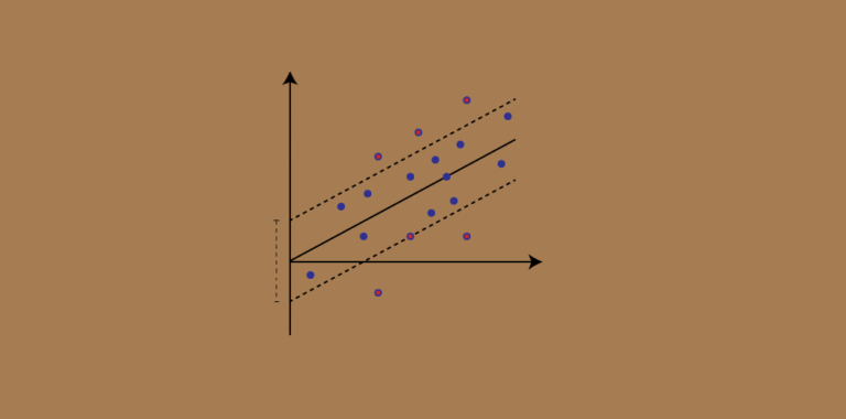
The key idea behind SVM is to find the optimal separating hyperplane that maximizes the margin between the two classes. The margin is defined as the distance between the hyperplane and the closest data points from each class. These closest points are called support vectors.

Mathematically, we want to find w and b such that:

wᵀxᵢ + b ≥ 1 for yᵢ = +1
wᵀxᵢ + b ≤ -1 for yᵢ = -1

where xᵢ is the i-th training example, and yᵢ is its corresponding class label.

These constraints ensure that the data points from each class lie on the correct side of the margin. The optimal hyperplane is the one that maximizes the margin while satisfying these constraints.

3. Primal Optimization Problem

To find the optimal hyperplane, we formulate an optimization problem. The objective is to maximize the margin, which is equivalent to minimizing the norm of the weight vector w. The optimization problem can be written as:

minimize ½ ||w||²
subject to yᵢ(wᵀxᵢ + b) ≥ 1 for i = 1, …, n

This is known as the primal optimization problem. The constraints ensure that each training example is correctly classified with a margin of at least 1.

4. Handling Non-Separable Data

In real-world scenarios, data is often not perfectly separable. To handle non-separable cases, we introduce slack variables ξᵢ that allow some data points to violate the margin constraints. The optimization problem becomes:

minimize ½ ||w||² + C Σ ξᵢ
subject to yᵢ(wᵀxᵢ + b) ≥ 1 – ξᵢ for i = 1, …, n
ξᵢ ≥ 0 for i = 1, …, n

The slack variables ξᵢ measure the extent to which a data point violates the margin constraint. The regularization parameter C controls the trade-off between maximizing the margin and minimizing the classification errors. A larger C value penalizes misclassifications more heavily, while a smaller C allows more flexibility in the margin.

5. Dual Formulation

Solving the primal optimization problem directly can be computationally challenging, especially when the number of features is large. To address this, we derive the dual formulation of the optimization problem using Lagrange multipliers.

The Lagrangian of the primal problem is:

L(w, b, ξ, α, β) = ½ ||w||² + C Σ ξᵢ – Σ αᵢ(yᵢ(wᵀxᵢ + b) – 1 + ξᵢ) – Σ βᵢξᵢ

where αᵢ and βᵢ are the Lagrange multipliers.

By setting the partial derivatives of the Lagrangian with respect to w, b, and ξᵢ to zero, we obtain the dual optimization problem:

maximize Σ αᵢ – ½ Σ αᵢαⱼyᵢyⱼ(xᵢᵀxⱼ)
subject to Σ αᵢyᵢ = 0
0 ≤ αᵢ ≤ C for i = 1, …, n

The dual problem is expressed in terms of the Lagrange multipliers αᵢ and involves the dot product between pairs of training examples xᵢᵀxⱼ.

6. Kernel Trick

One of the key advantages of SVM is its ability to handle non-linearly separable data by mapping the input features into a higher-dimensional space. However, explicitly computing this mapping can be computationally expensive or even infeasible.

The kernel trick allows us to implicitly compute the dot product in the higher-dimensional space without explicitly mapping the features. The dot product xᵢᵀxⱼ in the dual problem can be replaced by a kernel function K(xᵢ, xⱼ).

Popular kernel functions include:

• Linear Kernel: K(xᵢ, xⱼ) = xᵢᵀxⱼ
• Polynomial Kernel: K(xᵢ, xⱼ) = (γxᵢᵀxⱼ + r)ᵈ
• Radial Basis Function (RBF) Kernel: K(xᵢ, xⱼ) = exp(-γ||xᵢ – xⱼ||²)

The choice of kernel function depends on the problem and the underlying data distribution. The kernel function must satisfy certain properties, such as being symmetric and positive semi-definite.

7. Solving the Dual Problem

Once the dual optimization problem is formulated, it can be solved using quadratic programming techniques. The solution provides the optimal values of the Lagrange multipliers αᵢ.

The weight vector w can be expressed in terms of the Lagrange multipliers and the training examples:

w = Σ αᵢyᵢxᵢ

The bias term b can be computed using the Karush-Kuhn-Tucker (KKT) conditions.

8. Making Predictions

Given a new data point x, the predicted class label can be determined by evaluating the sign of the decision function:

f(x) = wᵀx + b = Σ αᵢyᵢK(xᵢ, x) + b

If f(x) ≥ 0, the predicted label is +1; otherwise, it is -1.

9. Support Vectors

The support vectors are the training examples that lie closest to the decision boundary and have non-zero Lagrange multipliers αᵢ. These points are critical in defining the optimal hyperplane and the margin.

Intuitively, the support vectors are the most informative and influential points in the training set. They provide the essential information needed to construct the SVM model.

10. Multi-Class SVM

While the basic SVM formulation is designed for binary classification, it can be extended to handle multi-class problems. Two common approaches are:

• One-vs-One (OvO): Train a separate binary SVM classifier for each pair of classes and use a voting scheme to determine the final class label.
• One-vs-Rest (OvR): Train a binary SVM classifier for each class, treating it as the positive class and all other classes as the negative class. Predict the class with the highest decision function value.

11. Advantages and Limitations

SVM offers several advantages:

• Effective in high-dimensional spaces
• Robust to outliers and noise
• Provides good generalization performance
• Kernel trick allows handling non-linearly separable data

However, SVM also has some limitations:

• Sensitive to the choice of kernel function and its parameters
• Training can be computationally expensive for large datasets
• Interpretability of the model can be challenging

12. Feature Scaling and Parameter Tuning

To achieve optimal performance with SVM, it is important to preprocess the input features by scaling them to a similar range. This helps in avoiding features with larger magnitudes dominating the optimization process.

Additionally, the choice of the regularization parameter C and the kernel parameters (e.g., γ for the RBF kernel) can significantly impact the model‘s performance. These parameters are typically tuned using techniques like cross-validation to find the best values for a given problem.

13. Applications of SVM

SVM has been successfully applied to a wide range of real-world problems, including:

• Text classification
• Image classification
• Bioinformatics
• Fraud detection
• Face recognition
• Handwritten digit recognition

Its ability to handle high-dimensional data and provide good generalization makes SVM a popular choice in many domains.

Conclusion

In this blog post, we explored the mathematical foundations of Support Vector Machines (SVM) for classification tasks. We discussed the representation of data in feature space, the concept of the optimal separating hyperplane, and the formulation of the primal and dual optimization problems.

We also covered the kernel trick, which allows SVM to handle non-linearly separable data, and discussed the role of support vectors in defining the decision boundary. Additionally, we touched upon multi-class SVM approaches, the advantages and limitations of SVM, and the importance of feature scaling and parameter tuning.

Understanding the mathematics behind SVM provides insights into its inner workings and helps in effectively applying and adapting the algorithm to various problems. With its strong theoretical foundations and practical applicability, SVM remains a valuable tool in the machine learning practitioner‘s toolkit.

I hope this blog post has shed light on the mathematical concepts underlying Support Vector Machines and has provided a deeper understanding of this powerful classification algorithm. Feel free to explore further resources and experiment with SVM on your own datasets to gain hands-on experience.

Happy learning and happy classifying!