Detecting Vehicle Motion with Background Subtraction using OpenCV

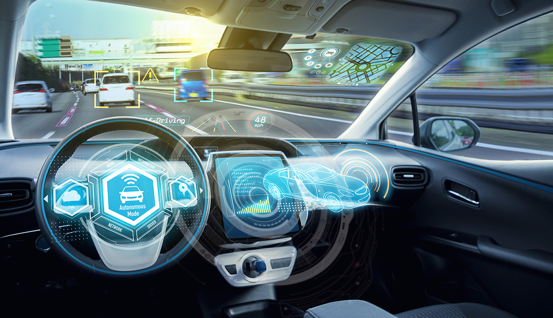
Vehicle detection is an important computer vision task with many real-world applications, from traffic monitoring to autonomous driving. One of the most effective techniques for identifying moving vehicles in a video stream is background subtraction. In this article, we‘ll take an in-depth look at using OpenCV‘s createBackgroundSubtractorMOG2 function to detect vehicle motion.

We‘ll cover the theory behind the technique and walk through a step-by-step code implementation, with considerations for parameter tuning and optimization. By the end, you‘ll have a solid foundation for applying background subtraction to your own vehicle detection projects. Let‘s dive in!

Applications of Vehicle Motion Detection

Vehicle detection has widespread applications across industries including transportation, public safety, and urban planning. Some common use cases include:

• Traffic monitoring and congestion analysis
• Vehicle counting and classification for highway planning
• Parking space occupancy detection and management
• Automated toll collection and enforcement
• Citywide traffic pattern modeling and optimization
• Pedestrian and cyclist safety systems
• Security and surveillance in sensitive areas
• Fleet tracking and logistics optimization

A 2020 report valued the global intelligent traffic management market size at over $20 billion, with expectations of significant continued growth driven by smart city initiatives and autonomous vehicle development.¹ Accurate, real-time vehicle detection plays a critical role in enabling these intelligent transportation systems.

Background Subtraction for Motion Detection

Background subtraction is a common computer vision technique for identifying moving foreground objects in video streams from static cameras. The key idea is to maintain a model of the background scene and then detect deviations from that model as foreground motion.

Mathematically, let $I(x, y, t)$ represent the intensity of a pixel at location $(x, y)$ and time $t$. We model the background intensity $B(x, y, t)$ and classify pixels as foreground if:

$|I(x, y, t) – B(x, y, t)| > \tau$

where $\tau$ is a predefined threshold. The main challenge is accurately modeling and updating the background over time as the scene changes.

Gaussian Mixture Model Background Subtraction

One of the most effective approaches is to model the background of each pixel as a mixture of $K$ Gaussian distributions. For pixel $(x, y)$, the probability of observing intensity $I_t$ at time $t$ is:

$P(It) = \sum{i=1}^K w_{i,t} \cdot \mathcal{N}(It | \mu{i,t}, \sigma_{i,t}^2)$

where $w{i,t}$, $\mu{i,t}$ and $\sigma_{i,t}$ are the weight, mean, and standard deviation of the $i$-th Gaussian component. The weights represent the proportions of past data accounted for by each component and sum to 1.

For each new frame, every pixel is checked against the existing $K$ Gaussian distributions. If a match is found with a Mahalanobis distance less than a threshold (typically 2.5), the pixel is classified as background and the component parameters are updated. If no match is found, the pixel is foreground, and the least probable distribution is replaced with a new one centered on the current intensity.

The MOG2 implementation in OpenCV, based on work by Zivkovic and van der Heijden², includes several enhancements over the original GMM formulation:

• Automatic selection of the number of components $K$ per pixel
• Adaptive learning rate for faster convergence
• Shadow detection to reduce foreground noise

These improvements help make the background model more robust to dynamic scene changes while still being computationally efficient to update.

Implementing MOG2 in OpenCV

OpenCV provides the createBackgroundSubtractorMOG2 function to easily apply Gaussian mixture model background subtraction to a video stream. Here‘s a step-by-step walkthrough of using it for vehicle detection.

Step 1: Initialize Video Capture and Background Subtractor

First, open a connection to the input video file or camera stream using cv2.VideoCapture. Then create the background subtractor object with the desired parameters:

import cv2

cap = cv2.VideoCapture(‘traffic.mp4‘)
fgbg = cv2.createBackgroundSubtractorMOG2(history=500, varThreshold=16, detectShadows=True)

• history is the number of frames used to build the background model. Higher values will adapt more slowly to changes but be more robust to momentary disturbances.
• varThreshold is a threshold on the squared Mahalanobis distance to decide if a pixel is foreground. A higher threshold will reduce false positives but may miss faint motion.
• detectShadows determines whether shadow pixels will be flagged differently than foreground. Disable for better performance if shadows are not important.

Step 2: Foreground Mask Generation and Cleanup

Next, loop through each frame of the video and apply the background subtractor to obtain a foreground mask:

while True:
    ret, frame = cap.read()
    if not ret:
        break

    fgmask = fgbg.apply(frame)

    kernel = cv2.getStructuringElement(cv2.MORPH_ELLIPSE, (5,5))
    fgmask = cv2.morphologyEx(fgmask, cv2.MORPH_OPEN, kernel)

The resulting fgmask is a grayscale image where white pixels (255) represent foreground motion, black pixels (0) are background, and gray pixels (127) are classified as shadows if enabled.

To remove noise and fill holes in the foreground mask, we apply a morphological opening operation with an elliptical kernel. This helps clean up the mask for more reliable vehicle segmentation.

Step 3: Vehicle Detection and Tracking

With the cleaned foreground mask, we can now extract individual vehicle regions using contour analysis. OpenCV‘s findContours function will identify connected regions of white pixels in the binary mask:

contours, _ = cv2.findContours(fgmask, cv2.RETR_EXTERNAL, cv2.CHAIN_APPROX_SIMPLE)

min_area = 400
vehicle_boxes = []
for contour in contours:
    if cv2.contourArea(contour) > min_area:
        x, y, w, h = cv2.boundingRect(contour)
        vehicle_boxes.append((x,y,w,h))

We filter the detected contours by area to ignore small patches of noise. The remaining regions are stored as bounding boxes representing potential vehicle detections for the current frame.

To track vehicles over time and handle momentary occlusions, we can match detections across frames based on bounding box overlap or more advanced algorithms like Kalman filtering. See the reference section for examples of multi-object tracking techniques that build on frame-level detections.

Step 4: Visualization and Analysis

With the vehicle regions identified, we can overlay bounding boxes on the input frame for visualization and extract useful statistics:

for (x,y,w,h) in vehicle_boxes:
    cv2.rectangle(frame, (x,y), (x+w,y+h), (0,255,0), 2)

cv2.putText(frame, f‘Vehicles: {len(vehicle_boxes)}‘, (30,30), 
            cv2.FONT_HERSHEY_SIMPLEX, 1, (0,0,255), 2)

cv2.imshow(‘Detected Vehicles‘, frame)

The green rectangles mark detected vehicles, while the red text displays a count of current detections, which could be logged over time for traffic volume analysis.

Additional statistics like average vehicle size, dominant trajectory directions, and lane-wise density could also be computed from the detection data and visualized or stored for further analysis.

Evaluation and Optimization

Assessing the accuracy of a vehicle detection pipeline can be challenging due to the lack of ground truth data in most scenarios. Common evaluation metrics applied to detection results include³:

• Precision: Percentage of detections that are true vehicles
• Recall: Percentage of true vehicles that are detected
• F1 score: Harmonic mean of precision and recall
• Intersection over union (IoU): Overlap between predicted and ground truth bounding boxes
• Mean average precision (mAP): Average precision over a range of recall thresholds

To quantify these metrics, manual annotation of some representative frames is usually required to establish a ground truth baseline. This can be a time-consuming process, so unsupervised measures like tracking consistency and trajectory smoothness are also used as proxy indicators of quality.

Depending on the specific application requirements, parameters like history, varThreshold, and min_area can be tuned to trade off between false positive and false negative detections. Other factors that can impact performance include:

• Illumination changes: Sudden lighting shifts from clouds, shadows, or headlights can disrupt the background model. Increasing history and enabling detectShadows can help to a degree.
• Camera jitter: Slight movements of the camera due to wind or vibration can register as false motion. Image stabilization techniques can be applied as a preprocessing step if needed.
• Low resolution: Vehicles that are too small in the frame may not have sufficient detail for motion segmentation. Using a higher resolution camera or focusing on a smaller field of view can improve results.
• Occlusion: Overlapping and partially-visible vehicles can be missed by background subtraction alone. Combining with an appearance-based classifier or part-based model can help.

Ultimately, the optimal configuration will depend on the specific deployment scenario and target performance level. It‘s recommended to test on a diverse set of representative videos and continuously monitor the output of a deployed system to catch potential failure cases.

Future Directions and Outlook

Background subtraction remains a widely-used technique for vehicle detection due to its simplicity and efficiency, but alternative paradigms are also being actively researched and applied:

• Appearance-based detection: Convolutional neural networks trained on large vehicle image datasets, like YOLO and Faster R-CNN, can detect vehicles based on visual features alone without requiring motion. These can be combined with background subtraction for improved robustness.

• Unsupervised anomaly detection: By learning a model of normal traffic patterns using autoencoders or GANs, unusual events like stopped vehicles or wrong-way drivers can be identified without explicit labeling. This is an active area of research for intelligent transportation systems.

• 3D object detection: Leveraging additional sensors like lidar and radar, vehicles can be detected and tracked in 3D space for a more complete view of the traffic scene. This is especially important for autonomous driving applications that require precise localization.

• Multi-object tracking: Advanced tracking algorithms like SORT⁴ and DeepSORT⁵ can be applied to link detections over time and handle challenges like occlusion and camera motion. This enables analysis of long-term traffic patterns and behaviors.

• Domain adaptation: Applying detectors trained on one dataset to a new location or camera setup can lead to performance drops. Techniques for adapting models to new domains with limited data are an important practical consideration.

As vehicle detection continues to advance, we can expect to see systems that are more accurate, efficient, and robust to real-world challenges. By combining multiple sensing modalities and leveraging large datasets and compute resources, the goal of truly reliable intelligent transportation is coming closer to reality.

Conclusion

In this article, we took a deep dive into the theory and practice of vehicle detection using the MOG2 background subtraction in OpenCV. We walked through the mathematical formulation, code implementation, and considerations for deployment and optimization.

The key things to take away are:

• Background subtraction is a powerful and efficient technique for detecting moving vehicles in static-camera video streams
• The MOG2 variant models each pixel as a mixture of Gaussians, allowing it to adapt to dynamic backgrounds and lighting changes
• OpenCV provides a high-level interface for applying MOG2 to a video stream in just a few lines of Python code
• Parameters like history and varThreshold can be tuned to trade off between detection sensitivity and noise
• Techniques for evaluating and optimizing vehicle detection systems include ground truth annotation, unsupervised quality measures, and continuous monitoring
• Alternative paradigms like appearance-based detection and 3D tracking are also active areas of research and deployment for vehicle detection

Whether you‘re a researcher exploring new techniques or a practitioner deploying a real-world system, the concepts and tools covered here should give you a strong foundation for understanding and applying vehicle detection. As always, feel free to experiment and adapt the code examples to your own needs – and happy detecting!

References

1. Markets and Markets. Intelligent Transportation System Market. https://www.marketsandmarkets.com/Market-Reports/intelligent-transport-systems-its-market-764.html
2. Z. Zivkovic and F. Van Der Heijden. Efficient adaptive density estimation per image pixel for the task of background subtraction. Pattern Recognition Letters, 27(7):773-780, 2006.
3. R. Padilla et al. A Comparative Analysis of Object Detection Metrics with a Companion Open-Source Toolkit. Electronics, 10(3):279, 2021.
4. A. Bewley et al. Simple Online and Realtime Tracking. IEEE International Conference on Image Processing (ICIP), 2016.
5. N. Wojke et al. Simple Online and Realtime Tracking with a Deep Association Metric. IEEE International Conference on Image Processing (ICIP), 2017.