Understanding the Basics of Artificial Neural Networks (ANNs)

Artificial neural networks (ANNs) are a powerful class of machine learning models loosely inspired by the structure and function of biological brains. Over the past decade, ANNs have achieved remarkable breakthroughs in areas like computer vision, natural language processing, and robotics. However, ANNs are sometimes seen as inscrutable "black boxes." In this post, we‘ll peel back the curtain and explain the core concepts behind these fascinating models. By the end, you‘ll have a solid grasp of how ANNs work and how to start building them yourself!

Brain Analogies and Biological Inspiration

ANNs are very simplified models of how the networks of neurons in animal brains process information. In brains, neurons are connected to each other in sprawling networks. Each neuron receives chemical and electrical signals from other neurons through branch-like structures called dendrites. If the total signal surpasses a certain threshold, the neuron "fires" and transmits the signal to other neurons via long fibers called axons. This simple mechanism of neurons activating based on inputs is the basis for all of the brain‘s incredible cognitive feats – perceiving the world, learning, making decisions, etc.

ANNs aim to loosely mimic this setup. They are made up of connected nodes (the "artificial neurons"), each of which does a simple computation based on inputs and passes the result to other nodes. This distributed, parallel processing allows ANNs to tackle complex problems.

Of course, ANNs are immense simplifications of biological neural networks. The human brain has around 86 billion neurons, each of which can have up to 10,000 connections! In comparison, even today‘s large ANNs have orders of magnitude fewer nodes and connections. Neurons also communicate via precisely timed electrical spikes, which ANNs don‘t model. Additionally, many details of how brains learn and encode information remain unknown. ANNs incorporate learnings from neuroscience, but are much more engineering tools than realistic brain models. Still, the brain metaphor is instructive for understanding ANNs at a high level.

Anatomy of an Artificial Neural Network

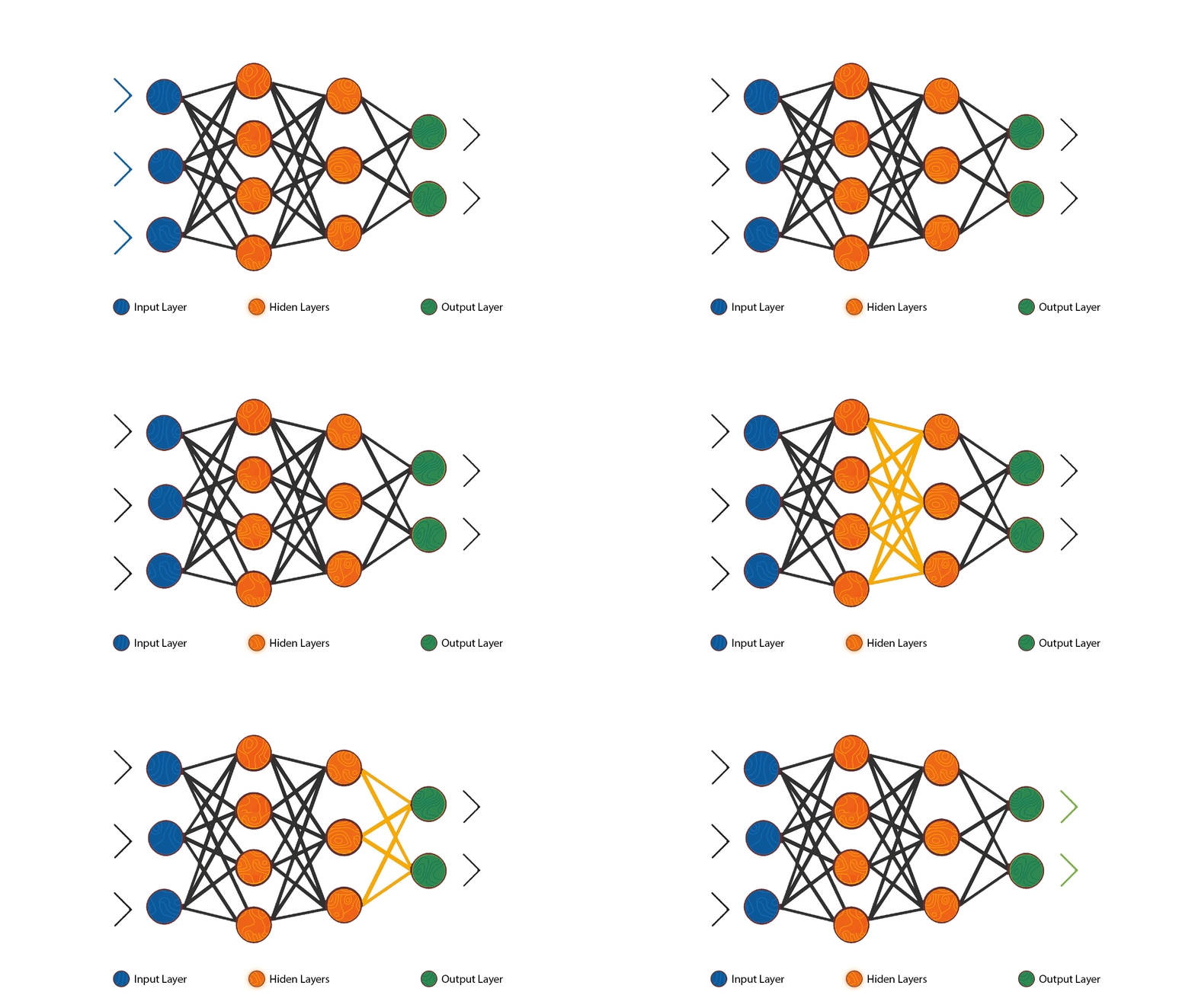
A basic ANN has a layered architecture, as shown in Figure 1. The first layer is the input layer, which accepts the data being fed into the network (e.g. images, text, numerical features). Each node in this layer corresponds to one input feature. The final layer is the output layer, which makes a prediction or decision (e.g. classifying an image). In between are one or more hidden layers that learn representations of the data. Information flows from the input layer, through the hidden layers, to the output layer.

[Include a diagram showing a basic 3-layer ANN architecture]

The nodes are the core processing units of the ANN. Each node has a set of incoming connections from nodes in the previous layer, and outgoing connections to nodes in the next layer. With each connection is associated a weight, which determines the strength of the signal that gets passed between nodes.

Here‘s what happens at each node during a forward pass through the network:

1. The node computes a weighted sum of all its inputs. Each input value is multiplied by the weight of the connection.
2. To this sum, a bias term is added. This allows the node to shift the input values.
3. The weighted sum plus bias is passed through an activation function. This function squashes the input into a certain range (usually between 0 and 1) and determines whether and to what extent the node "fires." Common activation functions include the sigmoid, hyperbolic tangent (tanh), and rectified linear unit (ReLU).
4. The node passes this activated value to all the nodes it‘s connected to in the next layer.

So in summary, each node computes: output = activation(weighted sum of inputs + bias). This simple computation is performed by every node in the network. Collectively, this allows the network to learn complex functions to map inputs to outputs. The magic lies in how the weights are gradually tuned to improve performance, which we‘ll cover next.

The Learning Process

The weights of an ANN are where the "intelligence" resides. Weights are typically initialized randomly. Then, through a training process called backpropagation, the weights are iteratively adjusted to minimize the network‘s error on a dataset. This allows the ANN to learn the optimal function for mapping inputs to outputs over many examples.

The training process goes as follows:

1. Forward propagation: A batch of training examples is fed through the network. Each node performs its weighted sum, bias add, and activation. This cascade of computations produces a final output for each example.

2. Calculating error: The network‘s outputs are compared to the true labels/values associated with each example. A loss function quantifies the error – common ones are mean squared error for regression and cross-entropy for classification. The goal is to minimize this loss.

3. Backpropagation: The error is "propagated backward" through the network. Using calculus, the amount each weight contributed to the final error is calculated. This is done using the chain rule to find the partial derivative (gradient) of the loss with respect to each weight.

4. Gradient descent: Each weight is nudged in the direction that minimizes the loss, determined by the gradient. The size of the update is determined by the learning rate hyperparameter.

Steps 1-4 are repeated many times on different batches of examples until the loss is minimized. There are various optimization algorithms used to speed up this process, like stochastic gradient descent (SGD), AdaGrad, and Adam.

In essence, backpropagation finds the optimal weights by exploring the high-dimensional "loss landscape." Nudging the weights in the direction of the negative gradient leads the network to a set of weights that minimize the loss on the training data. It‘s a bit like feeling your way down a hill in the dark – you keep taking steps in the direction of steepest descent until you reach the bottom.

Advantages and Applications of ANNs

ANNs have several properties that make them excellent general-purpose models:

• Ability to learn non-linear relationships: Many phenomena have complex, non-linear dynamics. ANNs can model these arbitrarily complex functions.

• Robustness to noise: ANNs are quite resistant to noisy or incomplete data.

• Scalability: ANNs can be scaled up to very deep/wide architectures to tackle highly complex problems given sufficient data and compute.

• Generalizability: A well-trained ANN can generalize to new, unseen data, allowing it to make good predictions on novel examples.

These advantages have led to transformative applications across many domains like:

• Computer vision: Convolutional neural networks (CNNs) can identify objects, faces, text, and more in images/video with human-like accuracy.

• Natural language processing (NLP): ANNs power language models like GPT-3 that can engage in fluent conversations, answer questions, and even write coherent essays.

• Recommendation systems: ANNs are used to recommend relevant content to users on platforms like YouTube, Netflix, and Spotify based on their history.

• Robotics: ANNs allow robots to process sensory inputs and make decisions for navigation, grasping, and other behaviors.

• Healthcare: ANNs can help detect diseases, predict health outcomes, and even discover new drugs.

• Finance: ANNs are used to detect fraud, make credit decisions, forecast financial markets, and more.

• Art and creativity: ANNs can generate striking artwork, music, and even video games in particular styles.

As data and computing power grow, ANNs are becoming increasingly pivotal in many industries. Their ability to find patterns in large, unstructured datasets is unmatched. Arguably, no technology will have a greater impact on the 21st century than AI systems built on neural networks.

Coding an ANN from Scratch

To cement your understanding, let‘s walk through how to code a basic ANN using Python and Keras, a popular deep learning library. We‘ll tackle a classic binary classification problem – predicting whether a patient has diabetes based on health measures.

First, we need to prepare the data:

from numpy import loadtxt
from keras.models import Sequential
from keras.layers import Dense

# load the dataset
dataset = loadtxt(‘pima-indians-diabetes.data.csv‘, delimiter=‘,‘)
# split into input (X) and output (y) variables
X = dataset[:,0:8]
y = dataset[:,8]

Here we load the Pima Indians Diabetes Dataset and split it into input features X and labels y.

Next, we define our model architecture:

# define the keras model
model = Sequential()
model.add(Dense(12, input_shape=(8,), activation=‘relu‘))
model.add(Dense(8, activation=‘relu‘))
model.add(Dense(1, activation=‘sigmoid‘))

We use the Keras Sequential model, which allows us to stack layers. Our simple model has three fully connected (Dense) layers:

• An input layer with 12 nodes, ReLU activation, and 8 input features
• A hidden layer with 8 nodes and ReLU activation
• An output layer with 1 node and sigmoid activation for our binary classification

This architecture allows the model to learn complex non-linear relationships between the input health metrics and the diabetes label.

We then compile the model by specifying the loss function, optimizer, and metrics to track:

# compile the keras model
model.compile(loss=‘binary_crossentropy‘, optimizer=‘adam‘, metrics=[‘accuracy‘])

For our binary classification problem, binary cross-entropy is an appropriate loss function. We use the Adam optimizer, which is known to work well for many problems.

Now we train the model on our data:

# fit the keras model on the dataset
model.fit(X, y, epochs=150, batch_size=10)

We run gradient descent for 150 epochs (passes through the dataset), with a batch size of 10 examples. With each epoch, the model adjusts its weights via backpropagation to minimize the loss.

Finally, we can evaluate the trained model‘s performance:

# evaluate the model
_, accuracy = model.evaluate(X, y)
print(‘Accuracy: %.2f‘ % (accuracy*100))

On this dataset, our simple model achieves ~75% accuracy at classifying patients as diabetic or not. Not bad for a few lines of code!

We can also use the trained model to make predictions on new, unseen data:

# make probability predictions with the model
predictions = model.predict(X)
# round predictions 
rounded = [round(x[0]) for x in predictions]

The model returns a probability between 0 and 1, which we can round to get a final classification.

There you have it – a working neural network! The same principles apply when building much larger, more sophisticated models. I encourage you to experiment with adding more layers, changing the number of nodes per layer, and tuning the optimization parameters.

Best Practices and Considerations

When working with ANNs, there are several key considerations and best practices to keep in mind:

• Preprocessing data: Cleaning, normalizing, and encoding data into an appropriate format before feeding it into the network is crucial.

• Splitting data: Data should be split into separate training, validation, and test sets. The validation set is used to evaluate the model during training and tune hyperparameters. The test set is used for final evaluation on unseen data.

• Overfitting: ANNs are prone to overfitting – performing very well on the training data but poorly on unseen data. Regularization techniques like dropout, L1/L2 regularization, and early stopping can help mitigate overfitting.

• Hyperparameter tuning: ANNs have many hyperparameters – number of layers/nodes, learning rate, activation functions, etc. These should be experimented with and tuned for optimal performance, typically using a validation set.

• Standardizing data: Subtracting the mean and dividing by the standard deviation of each feature can help the model learn appropriate weights faster and more stably.

• Monitoring loss and accuracy: During training, keep an eye on how the model‘s loss and accuracy evolve on both the training and validation sets. If the validation metrics start to stagnate or worsen while training metrics improve, the model may be overfitting.

Limitations and Future Directions

Despite their many strengths, ANNs have some notable limitations:

• Black box nature: The inner workings of ANNs can be difficult to interpret. Understanding how a network arrives at a particular prediction is an active area of research known as explainable AI (XAI).

• Data and compute requirements: ANNs typically require large amounts of labeled training data and significant computational resources, especially as models grow larger and more complex.

• Lack of generalization: ANNs can sometimes struggle to generalize to data that‘s very different from what they were trained on. Techniques like transfer learning aim to improve models‘ ability to adapt to new domains.

• Bias and fairness: ANNs can pick up on and amplify biases present in their training data, leading to unfair or discriminatory predictions. Ensuring AI systems are ethical and unbiased is a critical challenge.

• Robustness and security: ANNs can be fooled by adversarial examples – inputs specifically designed to cause misclassifications. Making models more robust to these kinds of attacks is an active area of research.

Despite these challenges, ANNs continue to evolve and achieve new breakthroughs. Some exciting areas of development include:

• Graph neural networks for modeling relational data like social networks and molecules
• Spiking neural networks that more closely mimic biological neurons‘ behavior
• Hybrid AI systems that combine ANNs with symbolic reasoning and knowledge bases
• Efficient neural networks that can run on resource-constrained devices like smartphones
• Lifelong learning systems that can continuously adapt to new tasks and environments

The field of neural networks is rapidly evolving, and we‘ve only scratched the surface of what‘s possible. As research continues, we can expect to see ANNs tackle ever more ambitious problems in more efficient and robust ways.

Conclusion

In this post, we‘ve covered the key concepts and mechanics underpinning artificial neural networks. We‘ve seen how ANNs take inspiration from biological brains, learning patterns and representations from data via iterative weight updates. While ANNs are extremely powerful and versatile tools, it‘s important to be aware of key challenges like overfitting and lack of interpretability. Still, ANNs will undoubtedly continue to drive breakthroughs in AI and shape the course of technological progress.

The code example walked through the key steps in building an ANN – preprocessing data, defining model architecture, training, and evaluation. I encourage you to dig deeper into the Keras documentation and experiment with building your own models!

I hope this post has demystified ANNs and given you a solid foundation for further exploration. The world of neural networks is fascinating and fast-moving – there‘s never been a more exciting time to dive in and start building intelligent systems. Happy learning!