An End-to-End Comprehensive Guide to Principal Component Analysis (PCA)

Introduction

Principal Component Analysis (PCA) is a fundamental technique in machine learning and data science for dimensionality reduction and feature extraction. It allows us to transform a high-dimensional dataset into a lower-dimensional space while retaining the most important information. PCA has wide-ranging applications, from image compression and customer segmentation to gene expression analysis and anomaly detection.

In this comprehensive guide, we will dive deep into the workings of PCA, exploring its mathematical foundations, step-by-step process, interpretation of results, and practical considerations. Whether you‘re a beginner looking to grasp the basics or an experienced practitioner seeking to enhance your understanding, this guide will provide you with the knowledge and tools to master PCA.

Mathematical Foundations of PCA

To understand PCA, we first need to grasp some key mathematical concepts. At the heart of PCA lies the covariance matrix, which captures the relationships between variables in a dataset. The covariance matrix is a square matrix where each element represents the covariance between two variables. A positive covariance indicates a positive relationship, while a negative covariance suggests an inverse relationship.

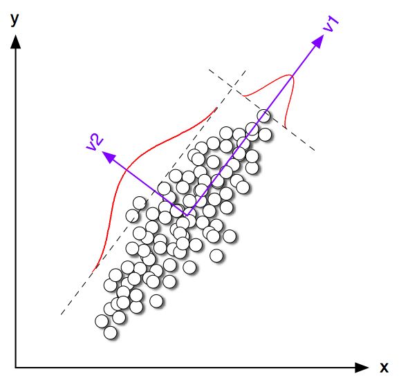
PCA relies on the eigendecomposition of the covariance matrix. Eigenvectors and eigenvalues are essential components of this decomposition. Eigenvectors represent the directions of maximum variance in the data, while eigenvalues quantify the amount of variance explained by each eigenvector. PCA seeks to find the eigenvectors with the largest eigenvalues, as they capture the most significant patterns in the data.

Another crucial concept in PCA is orthogonality. Orthogonal vectors are perpendicular to each other and have no correlation. PCA ensures that the principal components (eigenvectors) are orthogonal, allowing for a unique and interpretable representation of the data.

Step-by-Step PCA Process

Now that we have a foundation in the mathematics behind PCA, let‘s walk through the step-by-step process of performing PCA on a dataset.

Step 1: Data Standardization

Before applying PCA, it‘s essential to standardize the data. Standardization involves subtracting the mean and dividing by the standard deviation for each variable. This step ensures that all variables have zero mean and unit variance, preventing variables with larger scales from dominating the analysis.

Step 2: Computing the Covariance Matrix

Once the data is standardized, we compute the covariance matrix. The covariance matrix captures the relationships between variables and is calculated using the standardized data. The diagonal elements of the covariance matrix represent the variances of individual variables, while the off-diagonal elements represent the covariances between pairs of variables.

Step 3: Eigendecomposition

The next step is to perform eigendecomposition on the covariance matrix. Eigendecomposition reveals the eigenvectors and eigenvalues of the matrix. The eigenvectors represent the principal components, which are the directions of maximum variance in the data. The corresponding eigenvalues indicate the amount of variance explained by each principal component.

Step 4: Selecting Principal Components

After obtaining the eigenvectors and eigenvalues, we need to select the principal components to retain. This step involves deciding how many components to keep based on the desired level of dimensionality reduction. A common approach is to examine the scree plot, which shows the eigenvalues in descending order. The "elbow point" in the scree plot suggests the number of components to retain, as it represents the point where the explained variance starts to level off.

Step 5: Projecting Data onto Principal Components

Finally, we project the original data onto the selected principal components. This step transforms the data from the original high-dimensional space to a lower-dimensional space defined by the principal components. The projected data retains the most important information while reducing the dimensionality.

Interpreting PCA Results

Interpreting the results of PCA is crucial for gaining insights from the data. The scree plot, mentioned earlier, provides a visual representation of the explained variance by each principal component. By examining the scree plot, we can determine the optimal number of components to retain based on the desired trade-off between dimensionality reduction and preserved information.

Another important aspect of interpretation is the loading scores, which represent the contribution of each original variable to the principal components. Loading scores allow us to understand which variables have the most influence on each component. Variables with high absolute loading scores are strongly associated with the corresponding component.

Biplot visualization is a powerful tool for interpreting PCA results. A biplot displays both the observations and variables in the transformed space defined by the principal components. It allows us to visualize the relationships between variables and identify clusters or patterns in the data.

PCA Variants and Extensions

While the standard PCA is widely used, there are several variants and extensions that address specific challenges or accommodate different types of data.

Kernel PCA is an extension of PCA that can handle nonlinear relationships in the data. It maps the original data into a higher-dimensional feature space using a kernel function and then applies PCA in that space. Kernel PCA is particularly useful when the data has complex nonlinear structures.

Sparse PCA is another variant that aims to find principal components with sparse loading vectors. It is beneficial when dealing with high-dimensional data, as it helps identify a subset of relevant variables contributing to each component. Sparse PCA enhances interpretability and feature selection.

Incremental PCA is designed for streaming data or large datasets that cannot fit into memory. It allows updating the principal components incrementally as new data arrives, without recomputing the entire decomposition from scratch. Incremental PCA is computationally efficient and scalable.

Practical Considerations and Best Practices

When applying PCA in practice, several considerations and best practices should be kept in mind. Data preprocessing is a crucial step before performing PCA. This includes handling missing values, removing outliers, and scaling the data appropriately. Scaling ensures that variables with different units or ranges do not dominate the analysis.

Choosing the optimal number of components is another important consideration. While the scree plot provides guidance, it‘s often beneficial to experiment with different numbers of components and evaluate the results using cross-validation or domain knowledge.

Cross-validation helps assess the stability and generalization performance of PCA. It involves splitting the data into training and validation sets, performing PCA on the training set, and evaluating the reconstructed data on the validation set. This process helps prevent overfitting and ensures the robustness of the results.

It‘s also essential to be aware of the pitfalls and limitations of PCA. PCA assumes linearity in the data and may not capture complex nonlinear relationships. It is sensitive to the scale of the variables, emphasizing the importance of proper scaling. Additionally, PCA can be influenced by outliers, so robust preprocessing techniques should be employed.

Implementing PCA in Python

Python provides powerful libraries for implementing PCA, making it accessible to practitioners and researchers. The scikit-learn library is a popular choice for machine learning tasks, including PCA.

To implement PCA using scikit-learn, we first import the necessary modules:

from sklearn.decomposition import PCA
from sklearn.preprocessing import StandardScaler

Next, we standardize the data using the StandardScaler:

scaler = StandardScaler()
X_scaled = scaler.fit_transform(X)

Then, we create a PCA object, specifying the desired number of components:

pca = PCA(n_components=k)
X_pca = pca.fit_transform(X_scaled)

The fit_transform method fits the PCA model to the scaled data and returns the transformed data in the lower-dimensional space.

We can explore the explained variance ratio and the loading scores:

explained_variance_ratio = pca.explained_variance_ratio_
loadings = pca.components_

Visualizing the PCA results is often insightful. We can create a scree plot to visualize the explained variance:

import matplotlib.pyplot as plt

plt.plot(range(1, len(explained_variance_ratio) + 1), explained_variance_ratio, ‘bo-‘)
plt.xlabel(‘Principal Component‘)
plt.ylabel(‘Explained Variance Ratio‘)
plt.title(‘Scree Plot‘)
plt.show()

A biplot can be created to visualize the observations and variables in the PCA space:

plt.figure(figsize=(8, 6))
plt.scatter(X_pca[:, 0], X_pca[:, 1], color=‘blue‘, alpha=0.5)
plt.xlabel(‘PC1‘)
plt.ylabel(‘PC2‘)
plt.title(‘PCA Biplot‘)

for i, feature in enumerate(features):
    plt.arrow(0, 0, loadings[0, i], loadings[1, i], head_width=0.05, head_length=0.1, color=‘red‘)
    plt.text(loadings[0, i] * 1.15, loadings[1, i] * 1.15, feature, color=‘red‘, ha=‘center‘, va=‘center‘)

plt.show()

These code snippets provide a starting point for implementing PCA in Python. You can adapt and extend them based on your specific needs and dataset.

Case Studies and Real-World Examples

To solidify our understanding of PCA, let‘s explore some real-world examples and case studies.

Image Compression using PCA

PCA can be used for image compression by reducing the dimensionality of image data. By applying PCA to a set of images, we can extract the principal components that capture the most significant variations. By retaining only a subset of these components, we can compress the images while preserving the essential information. This technique is commonly used in computer vision and image processing applications.

Customer Segmentation in Marketing

In marketing, PCA can be employed for customer segmentation. By applying PCA to customer data consisting of various demographic and behavioral variables, we can identify the underlying patterns and group customers into distinct segments. These segments can be used to tailor marketing strategies, personalize recommendations, and improve customer targeting.

Gene Expression Analysis in Bioinformatics

PCA is widely used in bioinformatics for analyzing gene expression data. Gene expression datasets often have a high number of features (genes) compared to the number of samples. PCA can help reduce the dimensionality of the data, identifying the principal components that capture the most significant variations in gene expression patterns. This analysis aids in identifying co-expressed genes, discovering biological pathways, and understanding disease mechanisms.

Comparison with Other Dimensionality Reduction Techniques

While PCA is a popular dimensionality reduction technique, it‘s worth comparing it with other methods to understand their strengths and limitations.

t-SNE (t-Distributed Stochastic Neighbor Embedding) is a nonlinear dimensionality reduction technique that focuses on preserving the local structure of the data. Unlike PCA, t-SNE is particularly effective for visualizing high-dimensional data in a lower-dimensional space (usually 2D or 3D). However, t-SNE does not provide a direct mapping between the original features and the reduced dimensions, making it less interpretable compared to PCA.

LDA (Linear Discriminant Analysis) is another dimensionality reduction technique that is specifically designed for supervised learning tasks. While PCA seeks to maximize the variance in the data, LDA aims to maximize the separability between different classes. LDA finds linear combinations of features that best discriminate between the classes, making it suitable for classification problems.

Autoencoders are neural network-based models that can be used for dimensionality reduction. An autoencoder consists of an encoder network that maps the input data to a lower-dimensional representation and a decoder network that reconstructs the original data from the reduced representation. Autoencoders can learn nonlinear transformations and capture complex patterns in the data. However, they require careful design and training, and the reduced dimensions may not be as interpretable as those obtained from PCA.

Conclusion and Future Directions

In this comprehensive guide, we have explored the fundamental concepts, mathematical foundations, and practical applications of Principal Component Analysis (PCA). We discussed the step-by-step process of performing PCA, interpreting the results, and implementing it in Python. We also delved into PCA variants, practical considerations, and real-world examples.

PCA is a powerful tool for dimensionality reduction, feature extraction, and data visualization. It allows us to uncover hidden patterns, remove redundancies, and improve computational efficiency. However, it‘s essential to understand its assumptions, limitations, and the importance of data preprocessing.

As we move forward, there are several emerging trends and research areas in PCA. One direction is the development of robust PCA methods that can handle outliers and noise in the data. Another area of interest is the integration of PCA with deep learning architectures, such as convolutional neural networks, to learn hierarchical representations of data.

To further your understanding of PCA, I recommend exploring the following resources:

• "Pattern Recognition and Machine Learning" by Christopher M. Bishop
• "Elements of Statistical Learning" by Trevor Hastie, Robert Tibshirani, and Jerome Friedman
• scikit-learn documentation: https://scikit-learn.org/stable/modules/decomposition.html#pca
• "A Tutorial on Principal Component Analysis" by Jonathon Shlens

By mastering PCA and its applications, you can unlock valuable insights from high-dimensional data and tackle a wide range of machine learning and data science problems effectively.