The Ultimate Guide to Audio Classification Using Deep Learning
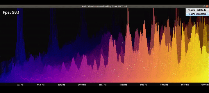
Audio classification is an exciting and rapidly evolving field that aims to automatically categorize and understand audio signals using machine learning techniques. It has a wide range of applications, from identifying different musical genres and instruments to detecting specific sounds in urban environments to classifying bird calls in nature. Over the past decade, deep learning approaches have achieved state-of-the-art performance on many audio classification tasks, surpassing traditional machine learning methods.
In this ultimate guide, we‘ll walk through the key concepts and techniques you need to know to get started with audio classification using deep learning. By the end, you‘ll have a solid foundation to tackle your own audio classification projects and deploy them in the real world. Let‘s dive in!
What is Audio Classification?
At its core, audio classification is the task of assigning a label or category to an input audio signal. The labels can represent high-level semantic concepts like music genres (e.g. classical, rock, hip hop), sound events (e.g. dog barking, glass breaking, gunshots), or even specific speakers or languages being spoken.
Traditionally, audio classification was done using hand-engineered features like mel-frequency cepstral coefficients (MFCCs) coupled with classical machine learning models such as support vector machines or random forests. However, with the rise of deep learning, we can now learn hierarchical representations directly from raw audio data that capture relevant patterns for the classification task at hand.
Deep Learning for Audio Classification
There are several deep learning architectures that have proven effective for audio classification:
Convolutional Neural Networks (CNNs): CNNs have been widely used for audio classification by treating the audio signal as a 2D image, with time on the x-axis and frequency on the y-axis. The convolution and pooling operations allow the model to learn local patterns and gradually build up higher-level representations. Popular CNN architectures for audio include SoundNet, M5, and the Deep Audio Classifier.
Recurrent Neural Networks (RNNs): RNNs are designed to handle sequential data and can capture temporal dependencies in audio signals. Variants like Long Short-Term Memory (LSTM) networks and Gated Recurrent Units (GRUs) help address the vanishing gradient problem. RNNs are often used in combination with CNNs, where the CNN acts as a feature extractor and the RNN models the temporal dynamics.
Transformer Models: Transformers have revolutionized natural language processing and are now being applied to audio tasks as well. Models like the Vision Transformer (ViT) and Audio Spectrogram Transformer (AST) treat the audio spectrogram as a sequence of patches and use self-attention mechanisms to model global dependencies. Transformers have achieved state-of-the-art results on several audio classification benchmarks.
Transfer Learning: Training deep learning models from scratch can be data and compute intensive. Transfer learning allows us to leverage pretrained models that have been trained on large-scale audio datasets and fine-tune them for our specific task with limited data. Popular pretrained audio models include OpenL3, PANN, and TRILL, which capture general-purpose audio representations.
Audio Preprocessing
Before feeding audio data into a deep learning model, we need to apply some preprocessing steps to convert the raw waveform into a suitable input representation. Here are some common techniques:
Resampling: Audio signals can have different sampling rates (e.g. 44.1 kHz for music, 16 kHz for speech). It‘s important to resample all audio inputs to a consistent sampling rate that the model expects.
Normalization: Audio signals can have varying amplitudes. Normalizing the waveform to a fixed range (e.g. [-1, 1]) helps the model learn more efficiently.
Mono Conversion: If the audio is stereo (2 channels), we can convert it to mono by averaging the channels. Most audio classification models operate on mono signals.
Spectrogram Extraction: The raw waveform is not directly suitable as input to CNNs. We typically compute a spectrogram, which is a visual representation of the frequency content of the signal over time. The most common type is the mel spectrogram, which applies a nonlinear frequency scaling to better match human perception. The mel spectrogram is treated as a 2D image input to the CNN.
Data Augmentation: To improve model robustness and generalization, we can apply data augmentation techniques to the audio signal or spectrogram. These include time stretching, pitch shifting, dynamic range compression, and adding background noise. SpecAugment and mixup are popular augmentation methods that have shown great success in audio classification.
Building an Audio Classifier in PyTorch
Now that we‘ve covered the basics, let‘s walk through building an audio classifier using PyTorch. We‘ll use the UrbanSound8K dataset, which contains 8732 labeled sound excerpts (<=4s) of urban sounds from 10 classes: air_conditioner, car_horn, children_playing, dog_bark, drilling, engine_idling, gun_shot, jackhammer, siren, and street_music.
First, we‘ll define a PyTorch Dataset class to load the audio files and apply the necessary preprocessing steps:
class UrbanSoundDataset(Dataset):
    def __init__(self, annotations_file, audio_dir, transformation, target_sample_rate, num_samples, device):
        self.annotations = pd.read_csv(annotations_file)
        self.audio_dir = audio_dir
        self.device = device
        self.transformation = transformation.to(self.device)
        self.target_sample_rate = target_sample_rate
        self.num_samples = num_samples

    def __len__(self):
        return len(self.annotations)

    def __getitem__(self, index):
        audio_sample_path = self._get_audio_sample_path(index)
        label = self._get_audio_sample_label(index)
        signal, sr = torchaudio.load(audio_sample_path)
        signal = signal.to(self.device)
        signal = self._resample_if_necessary(signal, sr)
        signal = self._mix_down_if_necessary(signal)
        signal = self._cut_if_necessary(signal)
        signal = self._right_pad_if_necessary(signal)
        signal = self.transformation(signal)
        return signal, label
This dataset will load the audio file, resample it to the target sampling rate, convert to mono, pad or trim to a fixed length, and apply the mel spectrogram transformation.
Next, we‘ll define a simple CNN architecture for classification:
class CNNNetwork(nn.Module):
    def __init__(self):
        super().__init__()
        self.conv1 = nn.Sequential(
            nn.Conv2d(
                in_channels=1,
                out_channels=16,
                kernel_size=3,
                stride=1,
                padding=2
            ),
            nn.ReLU(),
            nn.MaxPool2d(kernel_size=2)
        )
        self.conv2 = nn.Sequential(
            nn.Conv2d(
                in_channels=16,
                out_channels=32,
                kernel_size=3,
                stride=1,
                padding=2
            ),
            nn.ReLU(),
            nn.MaxPool2d(kernel_size=2)
        )
        self.conv3 = nn.Sequential(
            nn.Conv2d(
                in_channels=32,
                out_channels=64,
                kernel_size=3,
                stride=1,
                padding=2
            ),
            nn.ReLU(),
            nn.MaxPool2d(kernel_size=2)
        )
        self.conv4 = nn.Sequential(
            nn.Conv2d(
                in_channels=64,
                out_channels=128,
                kernel_size=3,
                stride=1,
                padding=2
            ),
            nn.ReLU(),
            nn.MaxPool2d(kernel_size=2)
        )
        self.flatten = nn.Flatten()
        self.linear = nn.Linear(128 * 5 * 4, 10)
        self.softmax = nn.Softmax(dim=1)

    def forward(self, input_data):
        x = self.conv1(input_data)
        x = self.conv2(x)
        x = self.conv3(x)
        x = self.conv4(x)
        x = self.flatten(x)
        logits = self.linear(x)
        predictions = self.softmax(logits)
        return predictions
This model has four convolutional layers for feature extraction, followed by a flatten and linear layer for classification. The softmax activation gives us a probability distribution over the 10 output classes.
Finally, we can train the model using the standard PyTorch training loop:
def train(model, data_loader, loss_fn, optimizer, epochs, device):
    for i in range(epochs):
        print(f"Epoch {i+1}")
        train_single_epoch(model, data_loader, loss_fn, optimizer, device)
        print("---------------------------")
    print("Finished training")

def train_single_epoch(model, data_loader, loss_fn, optimizer, device):
    for input, target in data_loader:
        input, target = input.to(device), target.to(device)

        # calculate loss
        prediction = model(input)
        loss = loss_fn(prediction, target)

        # backpropagate error and update weights
        optimizer.zero_grad()
        loss.backward()
        optimizer.step()

    print(f"loss: {loss.item()}")

def create_data_loader(train_data, batch_size):
    train_dataloader = DataLoader(train_data, batch_size=batch_size)
    return train_dataloader
We use a standard cross-entropy loss and the Adam optimizer. The training loop iterates over the dataset for a specified number of epochs, calculating the loss, backpropagating gradients, and updating the model weights.
After training, we can evaluate our model on a test set and use it to make predictions on new audio samples:
def predict(model, input, class_mapping):
    model.eval()
    with torch.no_grad():
        predictions = model(input)
        predicted_index = predictions[0].argmax(0)
        predicted = class_mapping[predicted_index]
    return predicted
Taking it Further
There are many ways to improve and extend this basic audio classification pipeline:
- Experiment with more advanced CNN architectures like ResNet or EfficientNet, or try using Transformer models like AST
- Apply transfer learning by using audio features extracted from pretrained models like OpenL3, PANN, or TRILL, and fine-tune on your target dataset
- Incorporate data augmentation techniques like SpecAugment and mixup to improve model robustness and generalization
- Deploy your trained model in a production environment using frameworks like TorchServe or CoreML
- Explore real-world applications of audio classification like acoustic monitoring, urban sound analysis, or music information retrieval
Conclusion
In this guide, we‘ve covered the key concepts and techniques behind audio classification using deep learning. We walked through the process of building an audio classifier in PyTorch, from data preprocessing to model architecture to training and inference.
Some key takeaways:
- Deep learning models like CNNs, RNNs, and Transformers have achieved state-of-the-art performance on audio classification tasks
- Mel spectrograms are a common input representation that captures both frequency and temporal information
- Data augmentation and transfer learning can significantly improve model performance and generalization
- PyTorch provides a flexible framework for building and training audio classification models
Audio classification is a rich and active area of research with many opportunities for innovation and real-world impact. By mastering the foundations and staying up-to-date with the latest advancements, you‘ll be well-equipped to tackle exciting audio classification projects and contribute to pushing the field forward.
To learn more, check out these great resources:
- [DCASE Challenge](http://dcase.community/) – Annual challenge on detection and classification of acoustic scenes and events
- [TorchAudio](https://pytorch.org/audio/stable/index.html) – PyTorch library for audio and signal processing
- [Papers with Code – Audio Classification](https://paperswithcode.com/task/audio-classification) – Collection of state-of-the-art papers and code on audio classification