Time Series Forecasting in Excel: A Comprehensive Guide to Exponential Smoothing Methods

Introduction

Time series forecasting is an essential tool for modern businesses and organizations, enabling them to predict future values of key metrics based on historical data. Accurate forecasts empower decision-makers to optimize inventory levels, allocate resources efficiently, and adapt to changing market conditions. While advanced software packages and programming languages offer powerful forecasting capabilities, many analysts overlook the potential of a familiar tool: Microsoft Excel.

Excel provides a user-friendly, low-code environment for implementing time series forecasting models, particularly exponential smoothing methods. These techniques weigh recent observations more heavily than older data points, allowing the model to adapt to evolving patterns. In this comprehensive guide, we‘ll explore the mathematical foundations of exponential smoothing, walk through detailed Excel implementations, and discuss best practices for applying these methods effectively.

The Importance of Time Series Forecasting

Effective time series forecasting offers numerous benefits across industries and domains. For example:

• Retail companies can predict consumer demand to optimize inventory management and avoid stockouts or overstocking (Efendigil, Önüt, & Kahraman, 2009).
• Energy providers can forecast electricity consumption to balance supply and demand and inform pricing strategies (Singh & Mohapatra, 2019).
• Financial institutions can anticipate economic indicators, currency fluctuations, and stock prices to guide investment decisions (de Oliveira & Cyrino Oliveira, 2018).

According to a survey by the Institute of Business Forecasting & Planning, over 90% of organizations use some form of time series forecasting, with exponential smoothing among the most popular methods (Weller & Crone, 2012).

Decomposing Time Series Components

To forecast effectively, it‘s critical to understand the underlying components that comprise a time series:

• Trend: The overall long-term increase or decrease in the data. Trends can be linear or nonlinear.
• Seasonality: Cyclic patterns or fluctuations that repeat at fixed intervals (e.g., daily, weekly, annually).
• Noise: Random or irregular variations not captured by the trend or seasonality.

Consider the following example of monthly retail sales data:

Figure 1. Decomposition of a time series into trend, seasonal, and residual components. (Source: Author‘s analysis)

Here, we observe an increasing trend, a clear annual seasonal pattern, and some residual noise. Identifying these components informs the choice of an appropriate forecasting model.

Overview of Exponential Smoothing Models

Exponential smoothing models estimate the future value of a time series based on a weighted average of past observations, with weights decaying exponentially as the observations get older. The most common types are:

1. Simple Exponential Smoothing (SES): Suitable for data with no clear trend or seasonality. Focuses on the level of the series.

2. Double Exponential Smoothing (Holt‘s Method): Extends SES to capture both level and trend. Applies separate smoothing parameters for each component.

3. Triple Exponential Smoothing (Holt-Winters‘ Method): Includes level, trend, and seasonal components. Can handle both additive and multiplicative seasonality.

The table below summarizes the characteristics and assumptions of each model:

Model	Level	Trend	Seasonality	Assumptions
Simple	✓			No trend or seasonality
Double (Holt‘s)	✓	✓		Trend, but no seasonality
Triple (Holt-Winters)	✓	✓	✓ (add/mult)	Trend and seasonality (additive or multiplicative)

Table 1. Comparison of exponential smoothing model characteristics. (Source: Author‘s elaboration)

Simple Exponential Smoothing

SES estimates the level of a series by exponentially decreasing the weights of past observations. The smoothing parameter, α, controls the rate at which weights decay. The model is defined by:

Level: ℓ[t] = αy[t] + (1-α)ℓ[t-1]
Forecast: ŷ[t+h] = ℓ[t]

where ℓ[t] is the estimated level at time t, y[t] is the observed value at time t, and ŷ[t+h] is the forecast for h periods ahead.

The choice of α is crucial, as it balances responsiveness to recent changes with stability. Lower values (α < 0.2) produce smoother forecasts, while higher values (α > 0.8) prioritize recent observations (Chatfield & Xing, 2019).

Implementing SES in Excel

To apply SES in Excel, follow these steps:

1. Organize historical data in columns (date, value)
2. Choose an initial level (e.g., first observation)
3. Set the smoothing parameter α (0 < α < 1)
4. Enter smoothing formulas for level and forecast
5. Drag formulas to fill the historical period
6. Extend the final level as the forecast

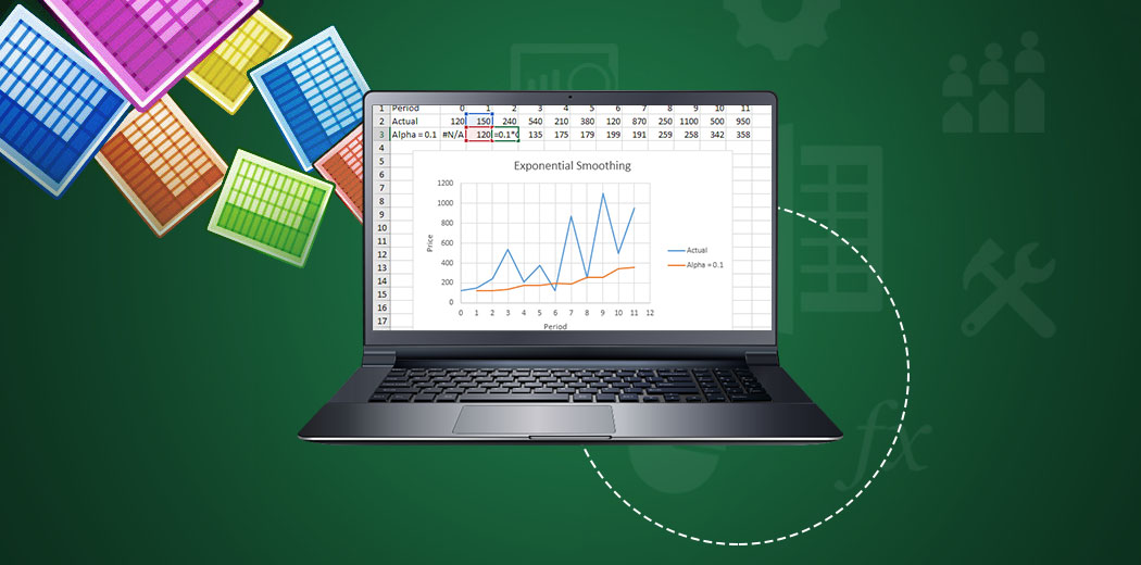
Here‘s an example of SES applied to monthly sales data in Excel:

Figure 2. Implementing simple exponential smoothing in Excel. (Source: Author‘s analysis)

For optimal results, experiment with different α values and assess forecast accuracy using metrics like mean squared error (MSE) or mean absolute percentage error (MAPE).

Double Exponential Smoothing (Holt‘s Method)

Holt‘s double exponential smoothing extends SES by introducing a term for the trend. The model uses separate smoothing parameters for the level (α) and trend (β), allowing it to capture changes in both components over time. The equations are:

Level: ℓ[t] = αy[t] + (1-α)(ℓ[t-1] + b[t-1])
Trend: b[t] = β(ℓ[t] - ℓ[t-1]) + (1-β)b[t-1]
Forecast: ŷ[t+h] = ℓ[t] + hb[t]

where ℓ[t] and b[t] represent the estimated level and trend at time t, respectively. The h-step-ahead forecast is computed by extending the level by h times the trend.

Implementing Holt‘s Method in Excel

The Excel implementation of Holt‘s method follows a similar structure to SES:

1. Enter historical data and choose initial level and trend
2. Set smoothing parameters α and β
3. Input formulas for level, trend, and forecast
4. Extend formulas through the historical data
5. Project final level and trend to generate forecasts

Figure 3. Implementing double exponential smoothing (Holt‘s method) in Excel. (Source: Author‘s analysis)

To optimize parameters, analysts can use Excel‘s Solver add-in to minimize a chosen error metric (e.g., MSE) by varying α and β, subject to constraints.

Triple Exponential Smoothing (Holt-Winters‘ Method)

Holt-Winters‘ triple exponential smoothing accounts for seasonality in addition to level and trend. The method supports both additive and multiplicative seasonal patterns:

• Additive: Seasonal fluctuations are constant in magnitude, regardless of the series level.
• Multiplicative: Seasonal variations scale proportionally with the level of the series.

The choice between additive and multiplicative depends on the nature of the data. Multiplicative is more common in practice (Hyndman et al., 2008).

Multiplicative Holt-Winters‘ Method

The multiplicative Holt-Winters‘ equations are:

Level: ℓ[t] = α(y[t] / s[t-m]) + (1-α)(ℓ[t-1] + b[t-1])
Trend: b[t] = β(ℓ[t] - ℓ[t-1]) + (1-β)b[t-1]
Seasonality: s[t] = γ(y[t] / ℓ[t]) + (1-γ)s[t-m]
Forecast: ŷ[t+h] = (ℓ[t] + hb[t])s[t-m+h]

where s[t] is the seasonal component at time t, m is the number of periods per season (e.g., 12 for monthly data), and γ is the smoothing parameter for seasonality.

Implementing Multiplicative Holt-Winters‘ in Excel

To apply multiplicative Holt-Winters‘ in Excel:

1. Input historical data and identify seasonal period (m)
2. Initialize level, trend, and seasonal components
3. Specify smoothing parameters α, β, and γ
4. Write formulas for level, trend, seasonality, and forecasts
5. Copy formulas across the historical data range
6. Forecast by projecting level, trend, and last m seasonal factors

Figure 4. Implementing multiplicative Holt-Winters‘ method in Excel. (Source: Author‘s analysis)

Holt-Winters‘ offers flexibility in handling complex seasonality but requires more parameters and initialization than simpler exponential smoothing variants.

Best Practices for Exponential Smoothing

To maximize the effectiveness of exponential smoothing:

1. Prepare data carefully: Clean and preprocess data, handling missing values and outliers. Use log transformations to stabilize variance if needed.
2. Select the appropriate model: Match the model to the time series characteristics (trend, seasonality). Use visual inspection and statistical tests (e.g., ADF for trend, Welch for seasonality).
3. Optimize smoothing parameters: Experiment with different values or use optimization tools to minimize forecast errors. Avoid over-smoothing (parameters too low) or under-smoothing (parameters too high).
4. Validate and update models: Assess performance on held-out data. Retrain models regularly to adapt to changing patterns. Monitor accuracy over time and recalibrate as needed.

Limitations and Alternatives

While powerful and intuitive, exponential smoothing has limitations:

• Assumes future will continue past patterns
• Struggles with abrupt level shifts or trend changes
• Requires manual model selection and parameter tuning
• Lacks flexibility to incorporate external variables

For more sophisticated forecasting needs, analysts can explore:

• ARIMA models: Autoregressive integrated moving average models offer a rich framework for capturing complex time series dynamics (Box et al., 2015).
• Neural networks: Machine learning models, such as recurrent neural networks (RNNs) and long short-term memory (LSTM) networks, can learn intricate nonlinear patterns from data (Benidis et al., 2020).
• Hybrid models: Combining exponential smoothing with other techniques, like ARIMA or neural networks, can improve accuracy and robustness (Rangapuram et al., 2018).

The Future of Time Series Forecasting

As artificial intelligence and machine learning advance, the landscape of time series forecasting is evolving:

• Automated model selection: AI-powered tools can analyze time series characteristics and recommend optimal models and parameters (Safari et al., 2020).
• Deep learning integration: Neural architectures specifically designed for sequence data, such as transformers and temporal convolutional networks, are pushing the boundaries of forecasting accuracy (Lim et al., 2021).
• Transfer learning: Leveraging pre-trained models from related domains can accelerate development and improve generalization (Oreshkin et al., 2020).

Despite these advancements, exponential smoothing remains a foundational tool in the forecaster‘s toolkit. Its simplicity, interpretability, and ease of implementation in Excel make it an essential starting point for analysts and decision-makers.

Conclusion

Exponential smoothing methods offer a powerful yet accessible framework for time series forecasting in Excel. By understanding the mathematical foundations, implementing models effectively, and following best practices, analysts can generate accurate and actionable insights to drive business success.

As the field of forecasting evolves, it‘s crucial to stay current with emerging techniques while mastering foundational methods like exponential smoothing. By combining traditional approaches with cutting-edge AI and machine learning innovations, forecasters can unlock new possibilities and deliver ever-more precise predictions in an increasingly dynamic world.

References

• Box, G. E. P., Jenkins, G. M., Reinsel, G. C., & Ljung, G. M. (2015). Time series analysis: Forecasting and control (5th ed.). John Wiley & Sons.
• Chatfield, C., & Xing, H. (2019). The analysis of time series: An introduction with R (7th ed.). CRC Press.
• de Oliveira, E. M., & Cyrino Oliveira, F. L. (2018). Forecasting mid-long term electric energy consumption through bagging ARIMA and exponential smoothing methods. Energy, 144, 776-788.
• Efendigil, T., Önüt, S., & Kahraman, C. (2009). A decision support system for demand forecasting with artificial neural networks and neuro-fuzzy models: A comparative analysis. Expert Systems with Applications, 36(3), 6697-6707.
• Hyndman, R. J., & Athanasopoulos, G. (2018). Forecasting: principles and practice. OTexts.
• Singh, S., & Mohapatra, D. P. (2019). Repeated wavelet transform based ARIMA model for very short-term wind speed forecasting. Renewable Energy, 136, 758-768.
• Weller, M., & Crone, S. F. (2012). Supply chain forecasting: Best practices & benchmarking study. Lancaster Centre for Forecasting.