Convolutional Neural Network Architecture: A Deep Dive

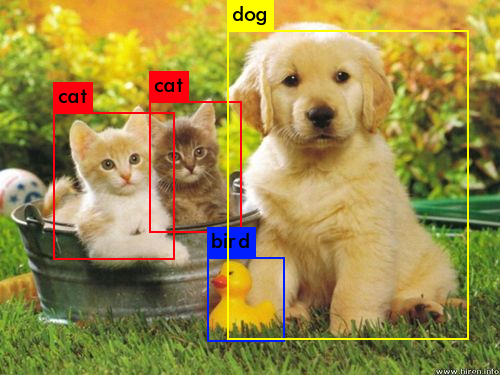
Convolutional Neural Networks (CNNs) have become the dominant approach for computer vision tasks since their groundbreaking success in the 2012 ImageNet competition. Drawing inspiration from the structure of the mammalian visual cortex, CNNs are designed to automatically learn hierarchical representations from raw pixel data. In this deep dive, we‘ll explore the key components of CNN architecture, understand how they work together to achieve powerful visual understanding, and survey the evolution of CNN designs that have pushed the state-of-the-art in image recognition.

Biological Inspiration

The architecture of Convolutional Neural Networks is inspired by the organization of the animal visual cortex, as discovered by Hubel and Wiesel in their seminal work in the 1950s and 1960s. They found that visual cortex contains a complex arrangement of cells, which are sensitive to small sub-regions of the visual field, called a receptive field. These cells act as local filters over the input space and are well-suited to exploit the strong spatially local correlation present in natural images.

Furthermore, they found that these receptive fields of different neurons partially overlap, to cover the entire visual field. This concept of receptive fields is what allows CNNs to learn spatial hierarchies of features – from simple edge detectors in early layers to more complex shapes and objects in later layers.

The Building Blocks of CNNs

At the core of the CNN architecture are three main types of layers: convolutional layers, pooling layers, and fully-connected layers. Let‘s dive into each of these in more detail.

Convolutional Layers

The convolutional layer is the fundamental building block of a CNN. The convolution operation is a specialized kind of linear operation that involves the multiplication of a set of weights (the filter or kernel) with the input, much like a traditional neural network. However, the key difference is that each filter is small spatially (along width and height), but extends through the full depth of the input volume.

Mathematically, for a 2D input $I$ and a 2D kernel $K$, the convolution operation $*$ is defined as:

$$(I*K)(i,j) = \sum_m \sum_n I(m,n) K(i-m, j-n)$$

Intuitively, the convolution operation slides the filter over the input, performing an element-wise multiplication and summing the results into the output pixel.

The output volume after a convolution will have a spatial size that depends on three parameters of the convolution operation:

• Depth: The number of filters used in the convolution.
• Stride: The number of pixels by which we slide the filter.
• Zero-padding: Padding the input volume with zeros around the border to control the spatial size of the output.

The spatial size of the output volume can be computed as a function of the input volume size $W$, the filter size $F$, the stride $S$, and the amount of zero padding $P$:

$$\frac{W-F+2P}{S} + 1$$

Pooling Layers

Pooling layers are used to reduce the spatial size of the representation, thus reducing the number of parameters and computation in the network. They operate independently on each depth slice of the input and resize it spatially. The most common form is max pooling, which reports the maximum output within a rectangular neighborhood. Other functions such as average pooling are also sometimes used.

Pooling helps to make the representation become invariant to small translations of the input – a small distortion in the input will not change the values of most of the pooled outputs. This is useful in computer vision because we want our classifications to be invariant to small translations and distortions in the input image.

Fully Connected Layers

After several convolutional and pooling layers, the final classification is done via fully connected layers. Neurons in a fully connected layer have full connections to all activations in the previous layer, as seen in regular neural networks. Their activations can hence be computed with a matrix multiplication followed by a bias offset.

The output from the final fully-connected layer is fed into a softmax function that converts the activations into class probabilities. The class with the highest probability is then chosen as the model‘s prediction.

Key Properties of CNNs

There are several key properties of CNNs that make them well-suited for image-related tasks:

Sparse Connectivity

Each neuron in a CNN is only connected to a small, localized region of the input volume, defined by the size of the convolutional filter. This sparse connectivity is in contrast to traditional neural networks where each neuron is connected to every neuron in the previous layer. This sparse connectivity not only reduces the number of parameters (and thus computational cost), but also reflects the intuition that spatially nearby pixels are more strongly related.

Parameter Sharing

In a traditional neural network, each element of the weight matrix is used exactly once when computing the output. In a CNN, each member of the kernel is used at every position of the input (except perhaps some boundary pixels, depending on the padding). This allows the network to look for a given feature everywhere in the input, allowing for translation invariance, and greatly reduces the number of parameters needed.

Equivariance

Convolutional layers have the property of equivariance to translation. This means that if the input image is shifted by a certain amount, the output of the convolutional layer will be shifted by the same amount, but will otherwise be unchanged. This property is desirable for image recognition tasks where we want the output to change predictably with respect to translations of the input.

The Evolution of CNN Architectures

Since the advent of AlexNet in 2012, there have been rapid advances in the design of CNN architectures. Here are some of the key milestones:

AlexNet (2012)

AlexNet, proposed by Alex Krizhevsky, was the first CNN to make a significant impact in the ImageNet Large Scale Visual Recognition Challenge (ILSVRC). It achieved a top-5 error of 15.3%, more than 10.8 percentage points lower than that of the runner up. The success of AlexNet sparked a renewed interest in CNNs in the computer vision community.

AlexNet featured five convolutional layers, some of which were followed by max-pooling layers, and three fully-connected layers with a final softmax. It used the non-saturating ReLU activation function which improved training speed. It also employed techniques like data augmentation and dropout to combat overfitting.

VGGNet (2014)

VGGNet, introduced by Simonyan and Zisserman, was the runner-up in ILSVRC 2014. Its main contribution was in showing that the depth of the network is a critical component for good performance. The team employed an architecture with very small (3×3) convolution filters, which allowed them to go deeper – up to 16-19 layers.

VGGNet demonstrated that deep networks with small filters can achieve state-of-the-art results. However, the network was computationally expensive, with 138M parameters for VGG-16.

GoogLeNet/Inception (2014)

GoogLeNet, developed by Szegedy et al. at Google, was the winner of ILSVRC 2014 with a top-5 error rate of 6.7%. Its main contribution was the development of the Inception module, which dramatically reduced the number of parameters in the network (4M, compared to AlexNet with 60M).

The idea of the Inception module is to have multiple sizes of filters (1×1, 3×3, 5×5) operating in parallel, which are then concatenated. This allows the network to capture features at multiple scales simultaneously. The 1×1 convolutions also help to reduce the dimensionality before the expensive 3×3 and 5×5 convolutions.

ResNet (2015)

Residual Networks (ResNets), introduced by He et al., were the winners of ILSVRC 2015 with an incredible error rate of 3.6%. ResNets are built from residual blocks where each block contains skip connections that bypass the non-linear transformations with an identity function.

The main insight of ResNets is that it is easier to optimize the residual mapping than to optimize the original, unreferenced mapping. Intuitively, it is easier to push the residual to zero than to fit an identity mapping by a stack of nonlinear layers.

ResNets are much deeper than previous architectures, using up to 152 layers while still having lower complexity than VGGNet. ResNets have become a cornerstone of many modern CNN architectures.

Beyond ResNet

Since ResNet, there have been numerous advancements in CNN architecture design. Some notable ones include:

• DenseNet (2017): Connects each layer to every other layer in a feed-forward fashion. This alleviates the vanishing-gradient problem, strengthens feature propagation, encourages feature reuse, and substantially reduces the number of parameters.

• SENet (2017): Introduces the "Squeeze-and-Excitation" (SE) block, which adaptively recalibrates channel-wise feature responses. This allows the network to perform feature recalibration, which can be seen as a form of attention.

• EfficientNet (2019): Developed through neural architecture search to optimize both accuracy and efficiency. EfficientNets achieve state-of-the-art accuracy on ImageNet while being much smaller and faster than previous models.

Here‘s a comparison of the performance and complexity of these architectures on the ImageNet dataset:

Architecture	Top-1 Accuracy	Top-5 Accuracy	Parameters (Millions)	GFLOPs
AlexNet	63.3%	84.6%	60	0.7
VGG-16	71.5%	90.1%	138	15.3
GoogLeNet	69.8%	89.6%	6.8	1.6
ResNet-50	77.2%	93.3%	25	3.9
DenseNet-121	74.9%	92.2%	7.9	2.9
SENet-50	77.6%	93.8%	27.7	4.1
EfficientNet-B0	76.3%	93.2%	4	0.4

*GFLOPs = Giga Floating Point Operations Per Second, a measure of computational complexity.

As we can see, modern architectures like ResNet, DenseNet, SENet, and EfficientNet significantly outperform earlier designs while being more parameter and computationally efficient.

Practical Considerations

When applying CNNs to real-world problems, there are several practical considerations to keep in mind:

Data Availability and Augmentation

CNNs typically require a large amount of training data to achieve good performance. When working with limited data, techniques like data augmentation (e.g., random cropping, flipping, rotating) can be used to artificially increase the size of the training set. Transfer learning, where a CNN pre-trained on a large dataset like ImageNet is fine-tuned on a smaller dataset, is also a powerful technique when data is scarce.

Overfitting and Regularization

CNNs, like all deep learning models, are prone to overfitting especially when training data is limited. Regularization techniques like L2 regularization, dropout, and early stopping should be used to combat overfitting. Batch normalization, which normalizes the activations of each layer, is also commonly used to improve training speed and reduce overfitting.

Hyperparameter Tuning

CNNs have many hyperparameters that need to be tuned for optimal performance, such as the number and size of filters, learning rate, batch size, etc. Techniques like grid search and random search can be used to find good hyperparameter settings. More advanced techniques like Bayesian optimization are also gaining popularity.

Computational Resources

Training deep CNNs can be computationally intensive, often requiring GPUs or even TPUs for efficient training. Inference (i.e., making predictions with a trained model) is less computationally expensive but can still be a bottleneck for real-time applications. Techniques like model compression and quantization can be used to reduce the computational cost of inference.

Conclusion

Convolutional Neural Networks have revolutionized the field of computer vision, achieving superhuman performance on tasks like image classification, object detection, and semantic segmentation. Their unique architecture, inspired by the structure of the visual cortex, allows them to automatically learn hierarchical representations from raw pixel data.

In this deep dive, we‘ve explored the key components of CNN architecture, including convolutional layers, pooling layers, and fully-connected layers. We‘ve seen how properties like sparse connectivity, parameter sharing, and equivariance make CNNs particularly well-suited for image-related tasks. We‘ve also traced the evolution of CNN architectures, from the seminal AlexNet to more recent designs like ResNet, DenseNet, and EfficientNet.

As the field continues to evolve, we can expect to see even more powerful and efficient CNN architectures emerge. However, it‘s important to keep in mind practical considerations like data availability, overfitting, hyperparameter tuning, and computational resources when applying CNNs to real-world problems.

Despite their success, CNNs are not a silver bullet. They struggle with tasks that require understanding of global context, reasoning, or interaction between objects. Techniques like capsule networks, graph convolutional networks, and transformers are being developed to address some of these limitations.

Nevertheless, Convolutional Neural Networks remain the workhorse of computer vision and a testament to the power of biologically-inspired artificial intelligence. As Yann LeCun, one of the pioneers of CNNs, said: "CNNs are the best example of biologically-inspired artificial intelligence. They are mathematically rigorous, computationally efficient, and have a wide range of applications. They are here to stay."